Seminar 5

Materials presented here build on the resources for instructors designed by Elena Llaudet and Kosuke Imai in Data Analysis for Social Science: A Friendly and Practical Introduction (Princeton University Press).

Seminar Objectives

This week, we will cover the following topics:

• Fitting a linear regression model with lm()
• Making predictions with predict()

Getting Started

1. Start by creating an R script to keep track of your code. In RStudio, you can open a new script by clicking File > New File > R Script.

2. Save your script by clicking File > Save As and saving it in your POL272 folder with the name seminar5.R.

3. Clear your environment to avoid operating with objects from previous work by mistake. You can do this by clicking on the broom icon in the Environment tab.

USArrests Dataset

We will use the USArrests dataset to practice fitting and interpreting linear regression models.

The USArrests dataset contains crime statistics for the 50 U.S. states in 1973, including:

• Murder: Number of murder arrests per 100,000 residents.
• Assault: Number of assault arrests per 100,000 residents.
• UrbanPop: Percentage of the population living in urban areas.
• Rape: Number of rape arrests per 100,000 residents.

Let’s first load the dataset and inspect it:

# Load the dataset
data("USArrests")

# View first few rows
head(USArrests)

           Murder Assault UrbanPop Rape
Alabama      13.2     236       58 21.2
Alaska       10.0     263       48 44.5
Arizona       8.1     294       80 31.0
Arkansas      8.8     190       50 19.5
California    9.0     276       91 40.6
Colorado      7.9     204       78 38.7

We are interested in predicting murder arrest rates using assault arrest rates. Therefore, we will be modeling the relationship between Assault, the predictor variable, and Murder, the outcome variable.

Exploratory Analysis

Let’s start by visualizing the relationship between Murder and Assault using a scatter plot:

# Load necessary package
library(ggplot2)

# Scatter plot of UrbanPop vs Murder
ggplot(USArrests, aes(x = Assault, y = Murder)) +
  geom_point(color = "blue") +
  labs(title = "Assault vs Murder Rates",
       x = "Assault Rate (per 100,000 residents)",
       y = "Murder Rate (per 100,000 residents)")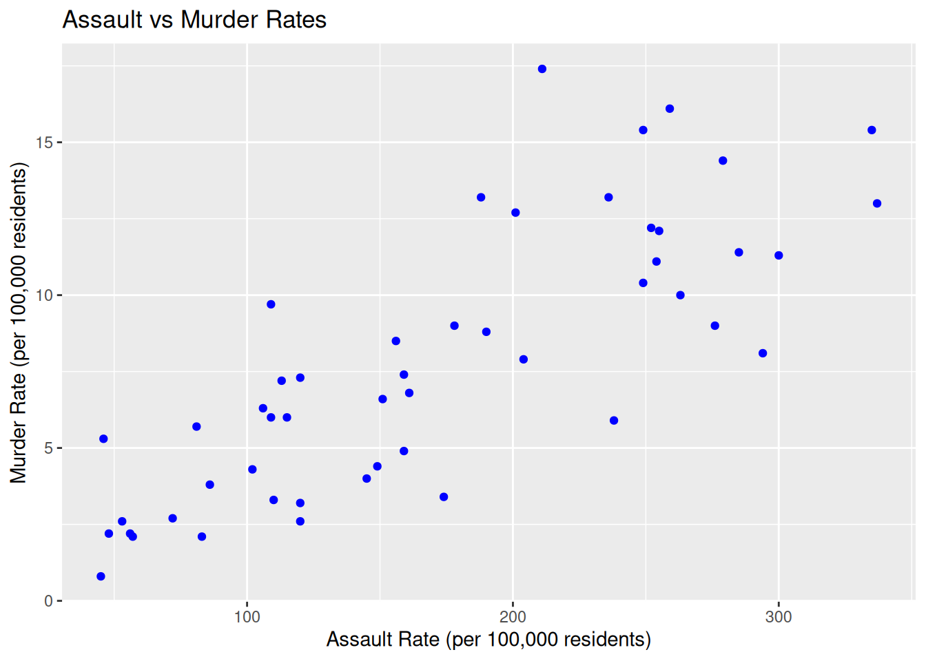

We can clearly see from our scatter plot that there is a strong, positive linear relationship between Assault and Murder.

To further investigate the direction and strength of the association between the two variables, we can compute the correlation coefficient using the function cor():

cor(USArrests$Assault, USArrests$Murder)

[1] 0.8018733

The correlation coefficient between the two variables turns out to be 0.8, which confirms what we noticed in the scatter plot above.

Fitting a Linear Regression Model

Now that we have a general sense of how the two variables relate to each other, we can fit a linear model to summarize their relationship. This is the model we will use later to make predictions.

Since our outcome of interest is Murder and our predictor is Assault, the line we want to fit is:

\[ \widehat{Murder}_i = \widehat{\alpha} + \widehat{\beta} \times Assault_i \quad \text{(i = states)} \]

where:

• \(\widehat{Murder}_i\): The predicted murder arrest rate for a state with a given assault arrest rate.

• \(Assault_i\): The observed assault arrest rate for state (i).

• \(\widehat{\alpha}\) (Intercept): The predicted murder arrest rate when Assault = 0.

• \(\widehat{\beta}\) (Slope): The change in the murder arrest rate for a one-unit increase in the assault arrest rate.

In simpler terms, this equation tells us: “If we know a state’s assault arrest rate, we can use this model to predict its murder arrest rate.”

The lm() function

To fit the model in R, we use the lm() function. The lm() function needs to know:

• The relationship we are trying to model (Murder ~ Assault)

• The dataset that contains our observations (data = USArrests)

To execute this, use the following code:

lm(Murder ~ Assault, data = USArrests)

Call:
lm(formula = Murder ~ Assault, data = USArrests)

Coefficients:
(Intercept)      Assault  
    0.63168      0.04191  

So here we have found that the line of best fit is given by:

\[ \widehat{Murder}_i = 0.63 + 0.042 \times Assault_i \]

Interpretation of the Intercept (0.63)

The intercept (0.63) represents the predicted murder arrest rate when the assault arrest rate is 0.

In simpler terms: If a state had zero assault arrests per 100,000 residents (which is highly unrealistic), the model predicts that the murder arrest rate would be 0.63 per 100,000 residents, on average.

Note: The interpretation of the intercept is often not meaningful in real-world terms because the dataset might never include cases where Assault is actually 0. This coefficient mainly ensures that the regression line fits the data properly.

Interpretation of the Slope (0.042)

The slope coefficient (0.042) tells us how the murder arrest rate changes when the assault arrest rate increases by one unit (one additional assault arrest per 100,000 residents).

In simpler terms: If assault arrests increase by 1 per 100,000 residents, murder arrests are expected to increase by 0.042 per 100,000 residents, on average.

The key takeaway: There is a positive relationship between assault and murder arrest rates. States with higher assault arrests tend to have higher murder arrests.

Making Predictions

1. Predicting Murder Rate for a Given Assault Rate

Let’s predict Murder when Assault = 200.

To do so, we simply substitute Assault = 200 into the regression equation:

\[ \widehat{Murder} = \widehat{\alpha} + \widehat{\beta} \times Assault \] \[ \widehat{Murder} = 0.63 + 0.042 \times 200 \] \[ \widehat{Murder} = 0.63 + 8.4 \] \[ \widehat{Murder} = 9.03 \]

To calculate this in R, we run:

# Compute predicted Murder arrest rate for Assault = 200
predicted_murder <- 0.63 + 0.042 * 200
predicted_murder

[1] 9.03

This means that if a state had 200 assault arrests per 100,000 residents, the predicted murder arrest rate would be 9.03 per 100,000 residents, on average.

The predict() function

Rather than calculating these values manually, we can also produce fitted values in R by using the predict() function. The predict function takes two main arguments:

• object: This is the model we created using lm(). It contains all the information R needs to make predictions.

• newdata: This is an optional argument where we tell R which values of the predictor (independent variable) we want predictions for.

  • If we don’t specify newdata, R will automatically calculate predictions for every observation in the dataset used to build the model.

  • If we do specify newdata, we need to provide a data frame where the column name matches the predictor in our model.

To execute this, we run:

# Store the linear model in an object
murder_assault_model <- lm(Murder ~ Assault, data = USArrests)

# Use predict() to compute the fitted value
predict(murder_assault_model, newdata = data.frame(Assault = 200))

       1 
9.013408 

2. Predicting the Change in Murder Rate for a Change in Assault Rate

Now, let’s predict how much the murder arrest rate would change if the assault arrest rate increased by 50 per 100,000 residents.

Using the slope coefficient (( = 0.042)), we compute:

\[ \Delta \widehat{Murder} = \widehat{\beta} \times \Delta Assault \] \[ \Delta \widehat{Murder} = 0.042 \times 50 \] \[ \Delta \widehat{Murder} = 2.1 \]

To calculate this in R, we run:

# Compute change in Murder rate for an increase in Assault by 50
murder_change <- 0.042 * 50
murder_change

[1] 2.1

This means that if the assault arrest rate increases by 50 per 100,000 residents, we expect the murder arrest rate to increase by 2.1 per 100,000 residents, on average.

✅ Key takeaway:

• The slope coefficient (0.042) tells us how much the murder arrest rate changes for each additional assault arrest per 100,000 residents.

• We omit the intercept in this calculation because we are not predicting an absolute murder arrest rate, only the change in the murder arrest rate.

Exercises

We are interested in predicting Assault using UrbanPop.

1. Visualize the relationship between Assault and UrbanPop using the ggplot2 package.

2. Use the lm() function to estimate a linear regression model, with UrbanPop as the predictor variable and Assault as the outcome variable. Store the fitted model in assault_urban_model for further analysis.

1. What is the estimated intercept? What does it represent?

2. What is the slope? How do you interpret it?

3. Predict the assault arrest rate for a state where UrbanPop = 60% using the predict() function.

4. If UrbanPop increases by 50 percentage points, how much would the assault arrest rate be expected to increase?

Solutions

1. Visualizing the relationship between Assault and UrbanPop:

ggplot(USArrests, aes(x = UrbanPop, y = Assault)) +
  geom_point(color = "blue") +
  geom_smooth(method = "lm", color = "red", se = FALSE) +
  labs(title = "Urban Population vs Assault Rates",
       x = "Urban Population (%)",
       y = "Assault Rate (per 100,000 residents)")

`geom_smooth()` using formula = 'y ~ x'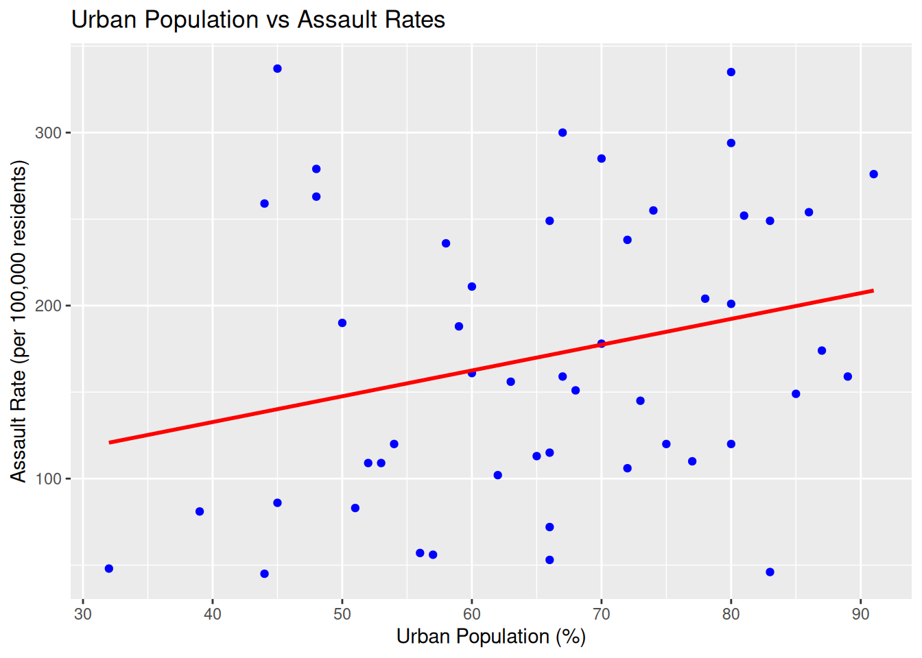

Interpretation: The plot shows a weak positive relationship between UrbanPop and Assault.

2. Fitting the linear regression model

assault_urban_model <- lm(Assault ~ UrbanPop, data = USArrests)
assault_urban_model #Print the results

Call:
lm(formula = Assault ~ UrbanPop, data = USArrests)

Coefficients:
(Intercept)     UrbanPop  
      73.08         1.49  

1. The estimated intercept (73.08) suggests that if the percentage of the population living in urban areas in a state was 0, the predicted assault arrest rate would be 73.08 per 100,000 residents, on average.

2. The slope (1.49) means that for every 1 percentage point increase in UrbanPop, the assault arrest rate is expected to increase by 1.49 per 100,000 residents, on average.

3. Predicting the assault arrest rate for UrbanPop = 60

predict(assault_urban_model, newdata = data.frame(UrbanPop = 60))

      1 
162.503 

4. Predicting change in Assault arrest rate when UrbanPop increases by 50:

1.49 * 50  

[1] 74.5

If UrbanPop increases by 50 percentage points, the assault arrest rate is expected to increase by 74.5 per 100,000 residents, on average. This follows directly from the slope coefficient: ( 1.49 = 74.5 ).