Seminar 4

Materials presented here build on the resources for instructors designed by Elena Llaudet and Kosuke Imai in Data Analysis for Social Science: A Friendly and Practical Introduction (Princeton University Press).

Seminar Objectives

This week, we will cover the following topics:

• Tables of frequency & proportion
• Histograms
• Descriptive statistics
• Scatter plots and correlation

Getting started

1. Start by creating an R script to keep track of your code. In RStudio, you can open a new script by clicking File > New File > R Script.

2. Save your script by clicking File > Save As and saving it in your POL272 folder with the name seminar4.R.

3. Clear your environment to avoid operating with objects from previous work by mistake. You can do this by clicking on the broom icon in the Environment tab.

4. Set the working directory by clicking on Session > Set Working Directory > Choose Directory. Navigate to your POL272 folder and click Open.

When you select the folder, RStudio will print the setwd(...) command in the Console. Copy and paste the command into your script so that R automatically sets the correct directory every time you run your script.

5. Load the “india.csv” dataset that you downloaded last week using the read.csv() function as shown below:

india <- read.csv("data/india.csv")

Frequency tables

The frequency table of a variable shows the values the variable takes and the number of times each value appears in the variable.

To create a frequency table in R, we use the function table(). The only required argument is the code identifying the variable to be summarised. For example, to calculate the frequency table of female, we run:

table(india$female)

  0   1 
214 108 

The frequency table shows that out of 322 villages in the dataset, 108 have a female politician (female == 1) and 214 have a male politician (female == 0).

Tidyverse Alternative: count()

We can achieve the same thing using the count() function from tidyverse:

library(tidyverse)

── Attaching core tidyverse packages ──────────────────────── tidyverse 2.0.0 ──
✔ dplyr     1.2.0     ✔ readr     2.1.6
✔ forcats   1.0.1     ✔ stringr   1.6.0
✔ ggplot2   4.0.2     ✔ tibble    3.3.1
✔ lubridate 1.9.5     ✔ tidyr     1.3.2
✔ purrr     1.2.1     
── Conflicts ────────────────────────────────────────── tidyverse_conflicts() ──
✖ dplyr::filter() masks stats::filter()
✖ dplyr::lag()    masks stats::lag()
ℹ Use the conflicted package (<http://conflicted.r-lib.org/>) to force all conflicts to become errors

india %>% 
  count(female)

  female   n
1      0 214
2      1 108

• india is the dataset.
• %>% is the pipe operator that passes india to the next function.
• count(female) counts the number of occurrences of each unique value in the female column.

Table of proportions

The table of proportions of a variable shows the proportion of observations that take each value in the variable. By definition, the proportions in the table should add up to 1 (or 100%).

To create a table of proportions in R, we use the function prop.table(), which converts a frequency table into a table of proportions. We can do this in two ways:

Option 1:

Create a frequency table first and assign it to an object:

table_female <- table(india$female)

Next, pass the object table_female as an argument to prop.table() to compute the proportions:

prop.table(table_female)

        0         1 
0.6645963 0.3354037 

Proportions can be transformed into percentages by multiplying by 100. Therefore, we can say that 66.46% (0.6645963 * 100, to 2 decimal places) of our sample is made up of villages that have male politicians (female == 0) and 33.54% (0.3354037 * 100, to 2 decimal places) of our sample is made up of villages that have female politicians (female == 1).

Option 2:

We can achieve the same thing by applying prop.table() directly to table():

prop.table(table(india$female))

        0         1 
0.6645963 0.3354037 

This one-liner creates and converts the table in a single step.

Tidyverse Alternative: mutate()

We can use count() to create a frequency table as we did before and then compute proportions using mutate() and prop.table().

india %>% 
  count(female) %>% 
  mutate(prop = prop.table(n)) 

  female   n      prop
1      0 214 0.6645963
2      1 108 0.3354037

Let’s break it down step by step:

• count(female) – This is the same function we used to create the frequency table before.

• mutate(prop = prop.table(n)) – Here, mutate() creates a new column called prop, which contains the proportion of villages in each category.

  • Note: The new column is only added to the results we see, not to the original dataset (india). The original data stays the same.

• prop.table(n) takes the column n (the frequency counts from count(female)) and converts it into proportions.

The result is the fraction of the total dataset that belongs to each category of female.

Histograms

A histogram is a graphical representation of the variable’s distribution, made up of bins (rectangles) of different heights. The position of the bins along the x-axis (the horizontal axis) indicates the interval of values. The height of the bins represents how often the variable takes the values in the corresponding interval.

The R function to create the histogram of a variable is hist(). For example, to produce the histogram of water, we simply run:

hist(india$water)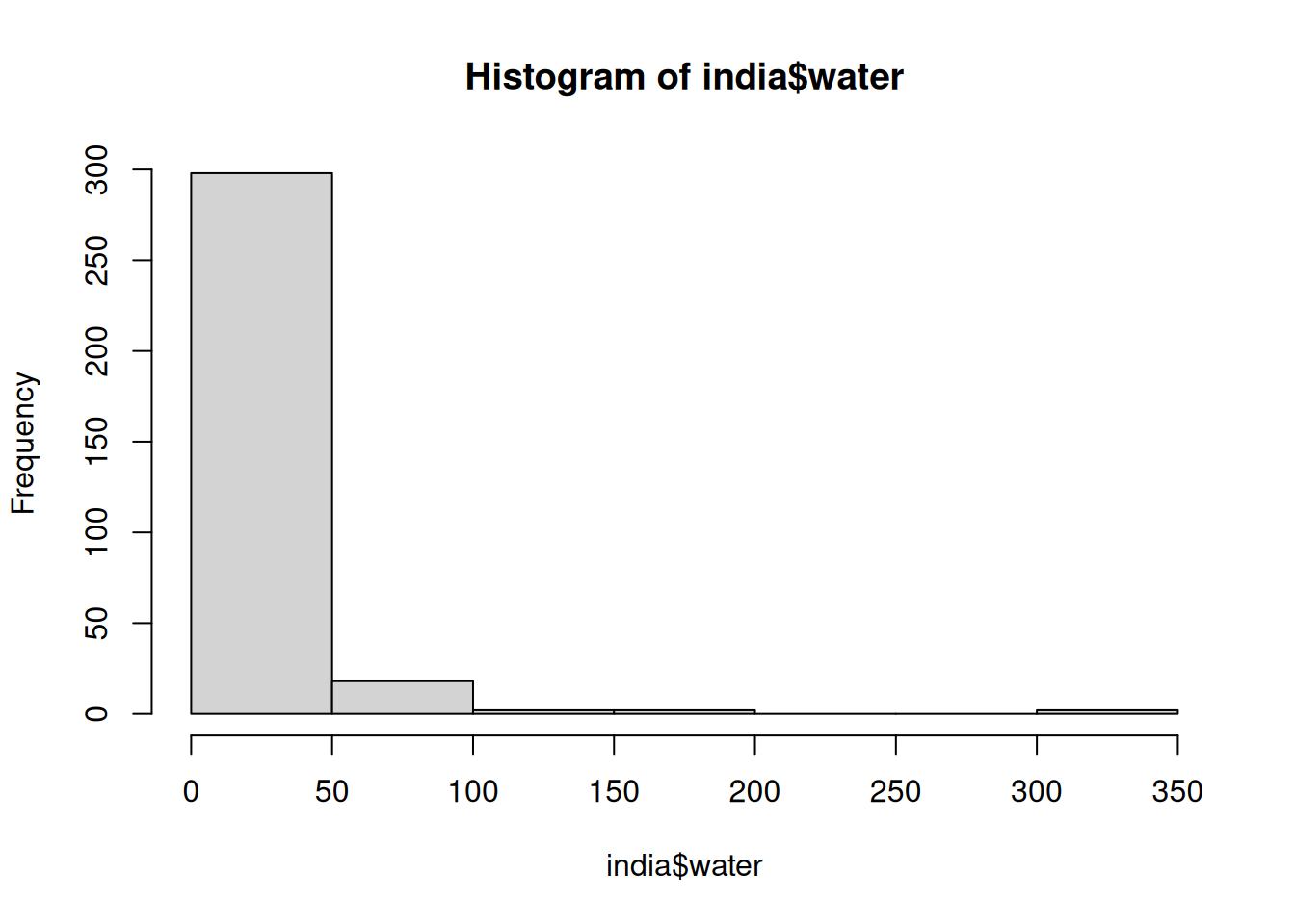

This will create a histogram where:

• The x-axis represents different intervals (bins) of water values.
• The y-axis represents the number of observations that fall into each bin.

After running this command, the histogram will appear in the Plots tab of RStudio (bottom-right panel by default).

Our histogram shows that the vast majority of the villages in our sample (more than 250 of the 322 villages) have had only a very small number of new (or repaired) water facilities built since random assignment. Only a tiny number of villages have had 50 or more new (or repaired) water facilities built. It is clear that the variable water does not follow a normal distribution, as it is highly skewed, with most values concentrated near zero and a long right tail representing a few villages with significantly more water facilities.

Tidyverse Alternative: ggplot2

We can create a histogram using ggplot2, which provides more customization options and a more structured approach to plotting.

library(ggplot2)

ggplot(data = india, aes(x = water)) + 
  geom_histogram()

`stat_bin()` using `bins = 30`. Pick better value `binwidth`.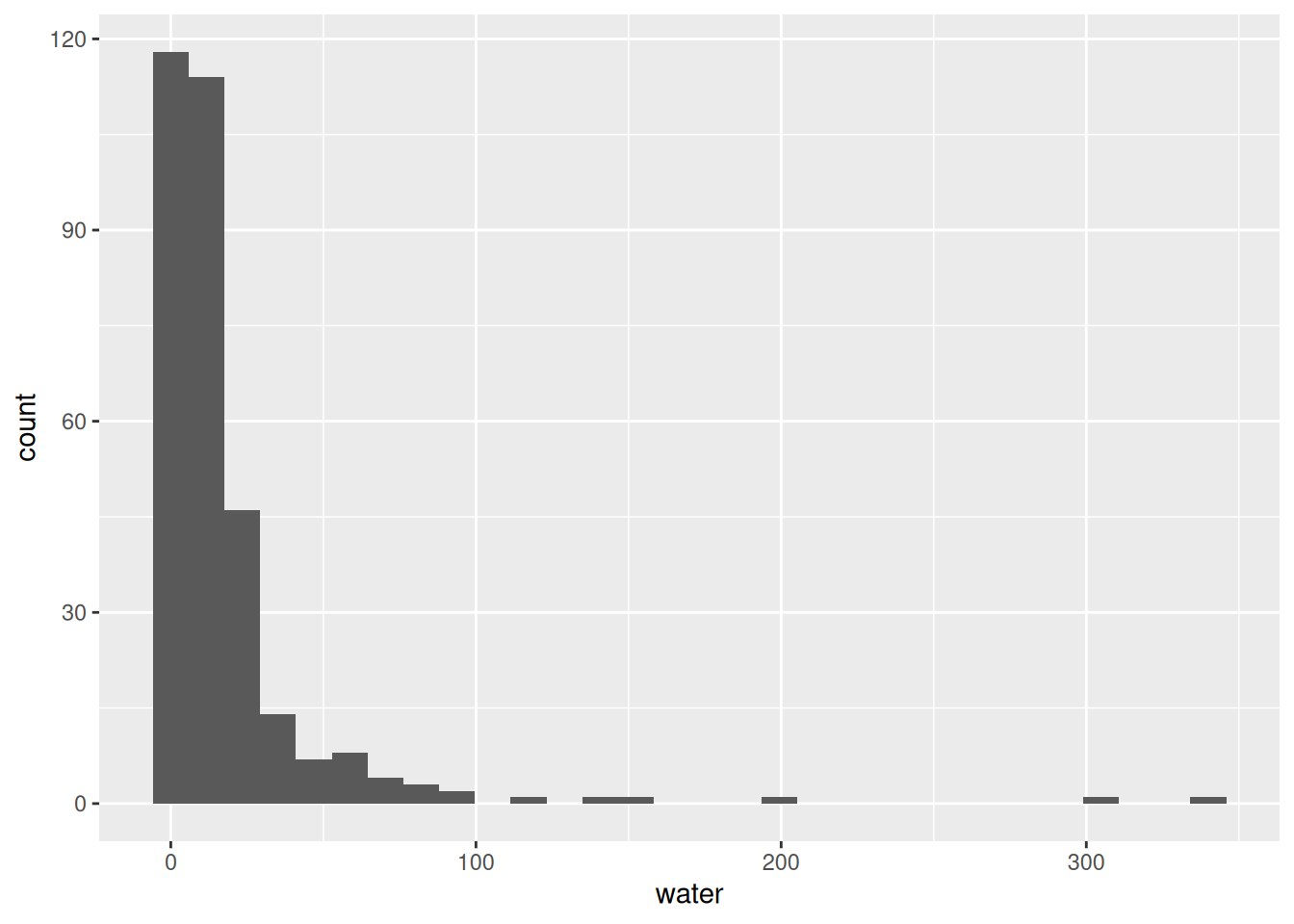

The ggplot() function takes two parameters.

• The first is the dataframe, here we use the dataframe india.

• The second specifies which columns of the dataframe we are looking to plot and onto which axis, using the aes() function. Here we map the column - or variable - water to the x-axis.

  • Simply specifying these two parameters will not draw our graph. To produce a histogram, we then need to add a histogram geometry to our code using the function geom_histogram().

Descriptive Statistics

Measures of centrality

Measures of centrality, such as the mean and the median, summarise the center of the distribution.

Mean

We’ve already seen multiple examples in weeks 1-3 on how to compute and interpret the mean of a variable. For example, using summarise(), we can compute the mean of water:

india %>% 
  summarise(mean_water = mean(water))

  mean_water
1   17.84161

Based on the results above, the average number of new (or repaired) water facilities is 18 per village.

Median

We can also describe the center of a distribution by using the median. The median is the value at the midpoint of the distribution that divides the data into two equal-size groups (or as close to it as possible). In other words, exactly half the values in the dataset will be smaller than the median and exactly half will be larger.

📝 Note: Calculating the median is important because it gives us an idea of the ‘typical’ value in the dataset, unlike the mean value which can be distorted by extreme values.

Using summarise(), we can compute the median of water as follows:

india %>% 
  summarise(median_water = median(water))

  median_water
1            9

The median value of 9 indicates that the typical village in our dataset had 9 new (or repaired) water facilities built since random assignment. In other words, half of the villages had 9 or fewer new (or repaired) water facilities, while the other half had more than 9.

Measures of spread

Measures of spread, such as the standard deviation and the variance, summarise the amount of variation of the distribution relative to its center.

Standard deviation

Standard deviation measures how spread out the values in a dataset are. A low standard deviation means most values are close to the average, while a high standard deviation means they vary widely.

Using summarise(), we can compute the standard deviation of water as follows:

india %>% 
  summarise(sd_water = sd(water))

  sd_water
1 33.67894

On average, the number of new (or repaired) water facilities in a village differs from the mean by about 33.68 facilities. This is a relatively large value (especially given the comparatively small size of this variable’s median and mean values), indicating that the range of our water values is large.

💡 Tip:

To determine whether the standard deviation is small or large, we compare it to the mean. This helps us understand how spread out the values are in the dataset.

• If the standard deviation is much smaller than the mean, the data points are closely clustered around the average (low variability).
• If the standard deviation is large compared to the mean, the data points are widely spread out (high variability).

A common way to assess relative variability is by calculating the coefficient of variation (CV), or the ratio of the standard deviation to the mean:

\[ CV = \left( \frac{\text{Standard Deviation}}{\text{Mean}} \right) \times 100 \]

We calculate the CV for water as follows:

cv_water <- (33.67894 / 17.84161) * 100

# Display results
cv_water

[1] 188.7663

The coefficient of variation (CV) = 188.77% tells us that the standard deviation is nearly twice the mean, meaning the values in water are highly dispersed relative to their average.

Variance

We sometimes use another measure of the spread of a distribution called variance. The variance of a variable is simply the square of the standard deviation.

Using summarise(), we can compute the variance of water as follows:

india %>% 
  summarise(var_water = var(water))

  var_water
1  1134.271

Alternatively, we can simply square the standard deviation for this variable which was returned above:

33.67894^2

[1] 1134.271

The variance of water is 1134. Again, this value is large, indicating a good deal of spread in the number of new (or repaired) water facilities built in our sample of villages since random assignment.

📝 Note: we are usually better off using standard deviations as our measure of spread, as they are easier to interpret because they are in the same unit of measurement as the variable.

Scatter plots

A scatter plot enables us to visualize the relationship between two variables by plotting one variable against the other in a two-dimensional space. Scatter plots are best for visualizing relationships between two non-binary numeric variables.

To create a scatter plot that shows the relationship between water and irrigation we run:

ggplot(data = india, aes(x = water, y=irrigation)) + 
  geom_point()

This code looks similar to the ggplot code used to produce the histogram above:

• We first specify our dataframe using the code data = india.

• We then specify the columns of the dataframe we are looking to plot and onto which axis, using the aes() function. Here we map the column - or variable - water to the x-axis and irrigation onto the y-axis.

• Finally, to produce our scatter plot, we add the point geometry to our code using the function geom_point().

📌 Does the linear relationship between these two variables look positive or negative?

• We see a positive linear relationship between our two variables. The slope of the line of best fit would be positive here. We can verify this by adding a line of best fit to our scatterplot like so:

ggplot(data = india, aes(x = water, y=irrigation)) + 
  geom_point() +
  geom_smooth(method = lm, se = FALSE)

`geom_smooth()` using formula = 'y ~ x'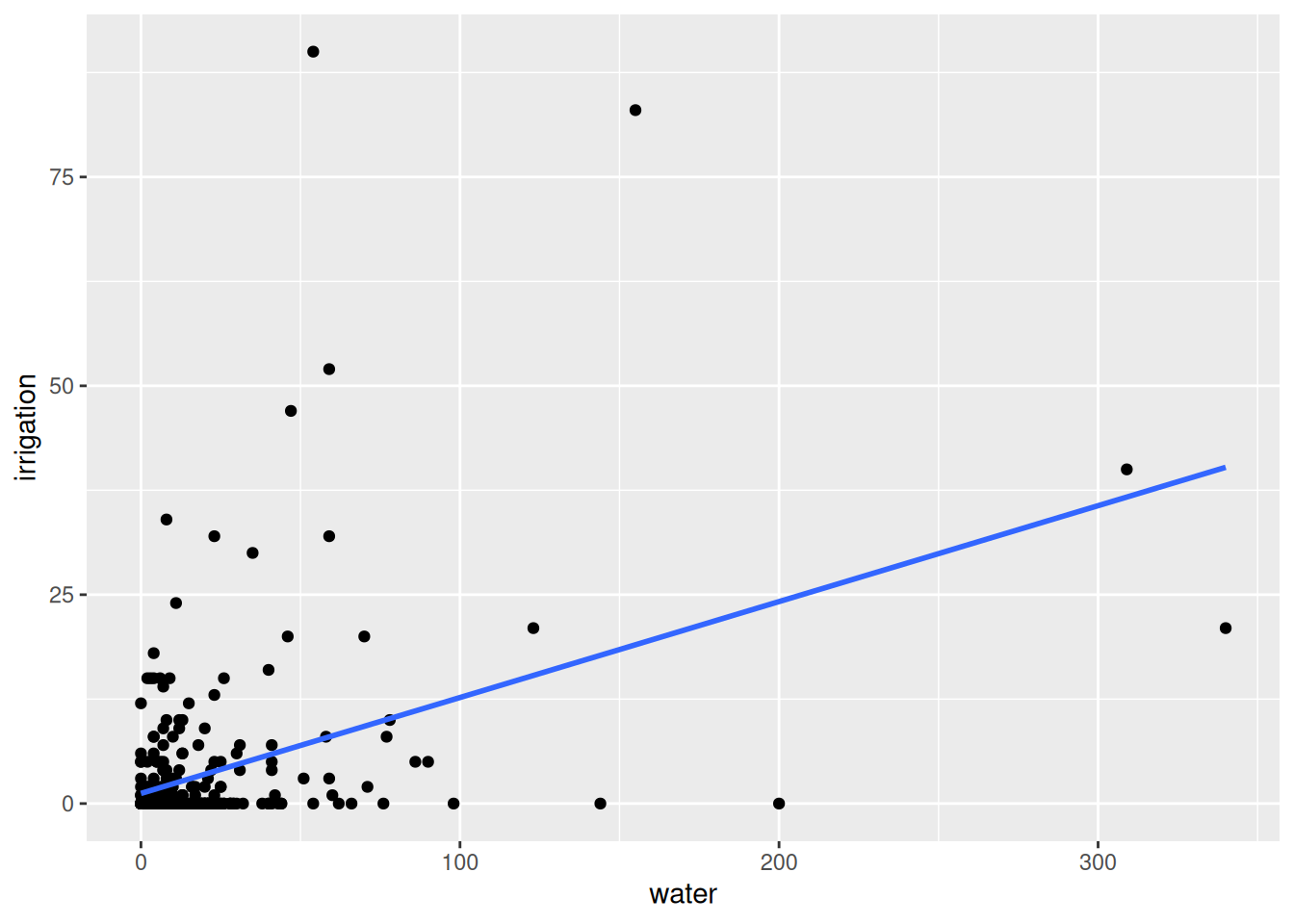

The code here is the same as for the previous scatter plot, it just adds the section geom_smooth(method=lm, se=FALSE) which asks R to draw a line of best fit on top of the original graph using the linear regression method and asks that the 95% confidence bounds of this line are not drawn.

📌 Does the relationship between these two variables look strong or weak?

• The relationship between these two variables does not look particularly strong. We can note that many of our observations are pretty far away from the line of best fit, which helps to explain the lacking strength of this relationship.

Correlation

While the scatter plot provides us with a visual representation of the relationship between two variables, sometimes it is helpful to summarise the relationship with a number. For that purpose, we use the correlation coefficient, or correlation for short.

We use the base R function cor() to compute the correlation of water and irrigation like so:

cor(india$water, india$irrigation)

[1] 0.4073307

The function cor() takes two arguments separated by a comma, this is the code identifying each variable to be used, and takes these in no particular order. You would get the same answer here if you switched the order of the variables water and irrigation.

Remember that the $ operator tells R to look for a column/variable within an object/dataframe.

📌 Questions

1. Are you surprised by the sign of the correlation?

Reveal Answer

We should not be surprised to see that the correlation between these variables is positive because, in the scatter plot above, we observe that the line that best summarises the relationship between them has a positive slope.

2. Are you surprised by the absolute value of the correlation?

Reveal Answer

Again, we should not be surprised that the absolute value of the correlation coefficient is 0.4 because, in the scatter plot above, we see that the relationship between water and irrigation does not appear to be overly strongly linear. The observations were pretty far away from the line of best fit.

3. If we wanted to use the sample of villages in this dataset to infer the characteristics of all villages in India, we would have to make sure that the sample is _____________ of the population. Please provide the missing word.

Reveal Answer

The missing word is representative. If we wanted to use the sample of villages in this dataset to infer the characteristics of all villages in india, we would have to make sure that the sample is representative of the population.

4. What would have been the best way of selecting the villages for the sample to ensure that the statement above was true?

Reveal Answer

The best way to make the sample of villages representative of all villages in india would have been to select the villages through random sampling.

Exercises

We will use the mtcars dataset to practice data visualisation, summary statistics, and correlation analysis. This dataset is built into R, and you can load it by simply running:

data(mtcars)

The data was extracted from the 1974 Motor Trend US magazine, and comprises fuel consumption and 10 aspects of automobile design and performance for 32 automobiles (1973–74 models). The variables are presented in Table 1 below.

Table 1: Variables in mtcars

Variable	Description
mpg	Miles/(US) gallon
cyl	Number of cylinders
disp	Displacement (cu.in.)
hp	Gross horsepower
drat	Rear axle ratio
wt	Weight (lb/1000)
qsec	1/4 mile time
vs	V/S
am	Transmission (0 = auto, 1 = manual)
gear	Number of forward gears
carb	Number of carburetors

1. Compute the proportion of cars by transmission type (am). What percentage of the cars in the dataset have manual transmission? What percentage have automatic transmission?

2. Create a histogram for Miles per Gallon (mpg). Interpret the distribution of the mpg variable. Does the mpg variable appear normally distributed?

3. Compute the mean, median, and standard deviation for mpg using the summarise() function. Interpret the results.

4. Plot the relationship between mpg and wt using a scatter plot and add a line of best fit. Is the relationship positive or negative? Would you say the relationship is strong or weak?

5. Compute the correlation between mpg and wt. Does it match what you observed in the scatter plot?

Solutions

1. Compute the proportion of cars by transmission type:

prop.table(table(mtcars$am))

      0       1 
0.59375 0.40625 

Interpretation: 59.38% of cars have automatic transmission (am = 0), and 40.63% have manual transmission (am = 1). The dataset has more automatic cars than manual.

2. Create a histogram for mpg:

library(ggplot2)

ggplot(data = mtcars, aes(x = mpg)) + 
  geom_histogram(binwidth=3)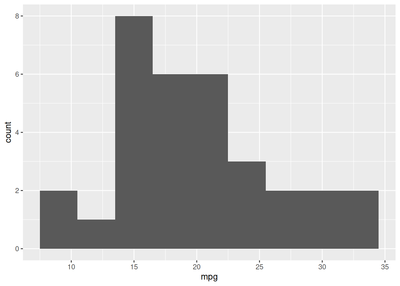

📝 Note: To improve readability, setting binwidth = 4 (or another reasonable value) creates wider bins, smoothing the histogram and making the overall shape easier to interpret.

The histogram shows the frequency of cars within different MPG ranges. The variable is not normally distributed, but instead appears slightly right-skewed, meaning there are more cars with lower MPG (around 15-20 MPG), but a few models exhibit very high MPG (above 30 MPG).

3. Compute the mean, median, standard deviation, and variance for mpg:

mtcars %>% 
  summarise(
    mean_mpg = mean(mpg),
    median_mpg = median(mpg),
    sd_mpg = sd(mpg)
  )

  mean_mpg median_mpg   sd_mpg
1 20.09062       19.2 6.026948

Interpretation:

• Mean (20.09): The average car gets 20.09 miles per gallon.
• Median (19.2): Half of the cars get less than 19.2 mpg, and half get more.
• Standard Deviation (6.03): On average, mpg values differ from the mean by about 6 mpg. Since the standard deviation (6.03) is about 30% of the mean, this suggests moderate variability in fuel efficiency across the dataset.

4. Scatter plot of mpg vs. wt:

ggplot(data = mtcars, aes(x = mpg, y = wt)) + 
  geom_point() +
  geom_smooth(method = lm, se = FALSE, color = "red") 

`geom_smooth()` using formula = 'y ~ x'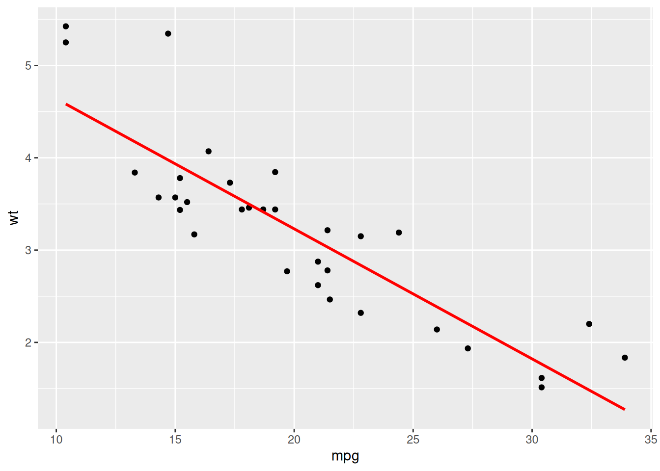

The relationship is negative. As miles per gallon (mpg) increases, weight (wt) decreases. The points are closely clustered around the line, meaning the relationship is strong.

5. Compute the correlation between mpg and wt:

cor(mtcars$mpg, mtcars$wt)

[1] -0.8676594

This is a strong negative correlation, as observed in the scatter plot.