Week 11: Assumptions of Linear Regression
POL272 Quantitative Methods for Social Science Research
Assumption 1: \(E(u_i|X_i) = 0\)
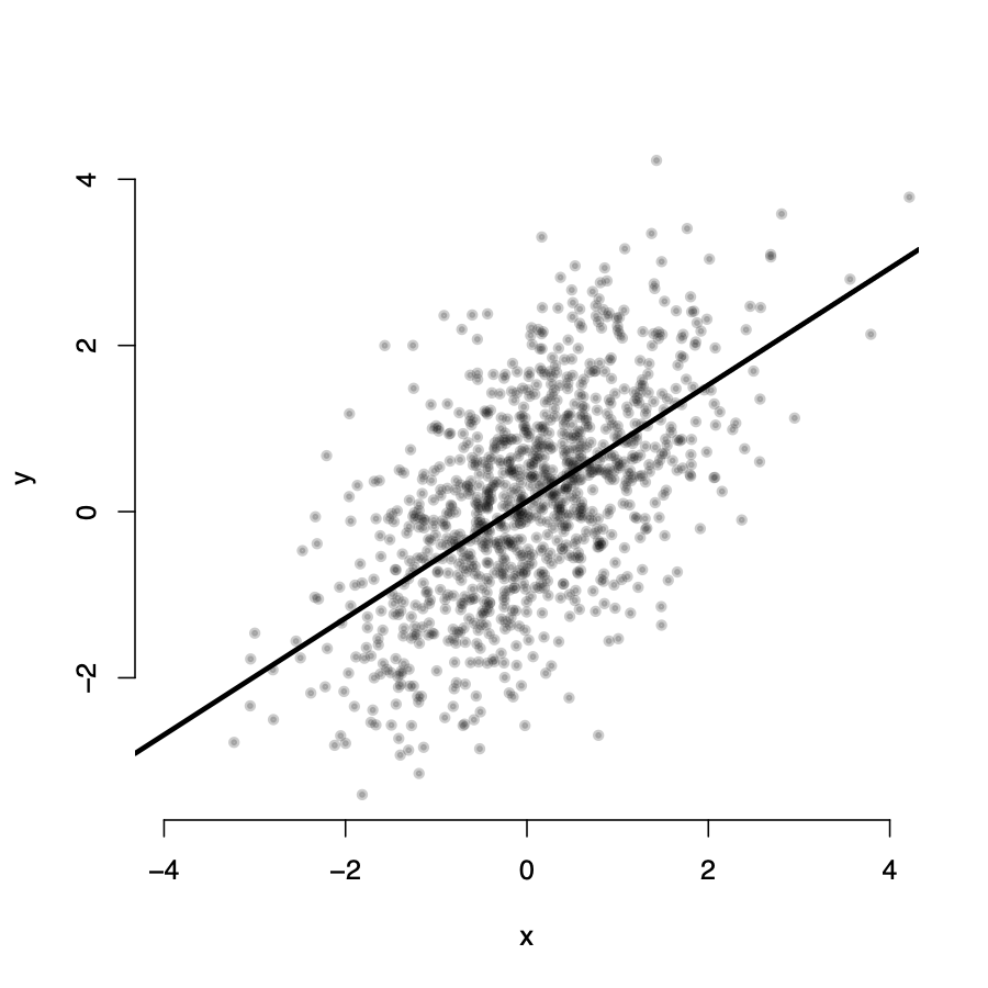
Assumption 1: \(E(u_i|X_i) = 0\)

Assumption 1: \(E(u_i|X_i) = 0\)
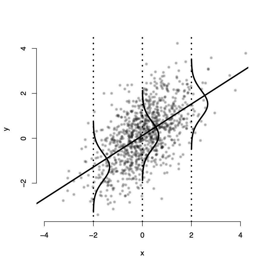
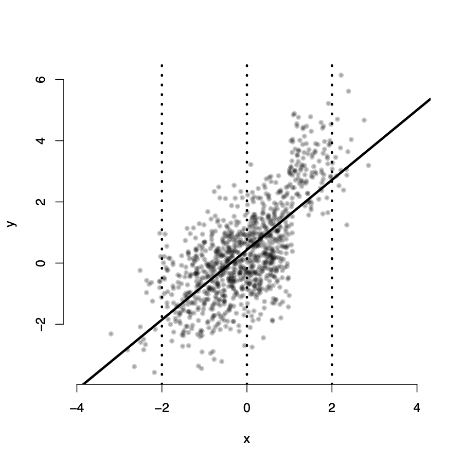
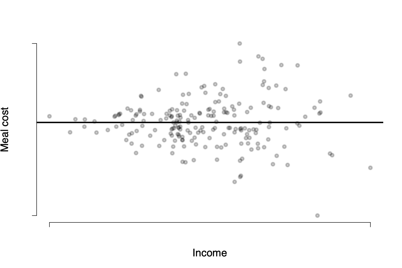
\(Y_i\) seems randomly distributed around the line for all values of X
\(\rightarrow\) in expectation, for any value \(X_i\), the value of \(u_i = 0\)
Assumption 1: \(E(u_i|X_i) \neq 0\)
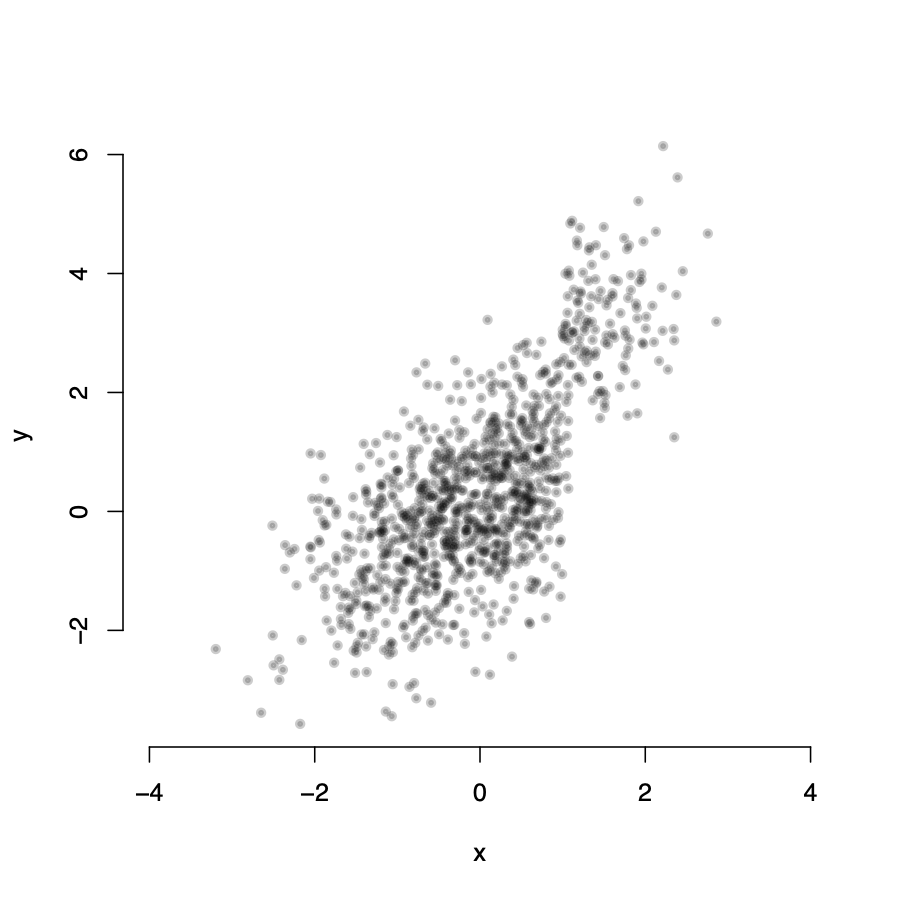
Assumption 1: \(E(u_i|X_i) \neq 0\)
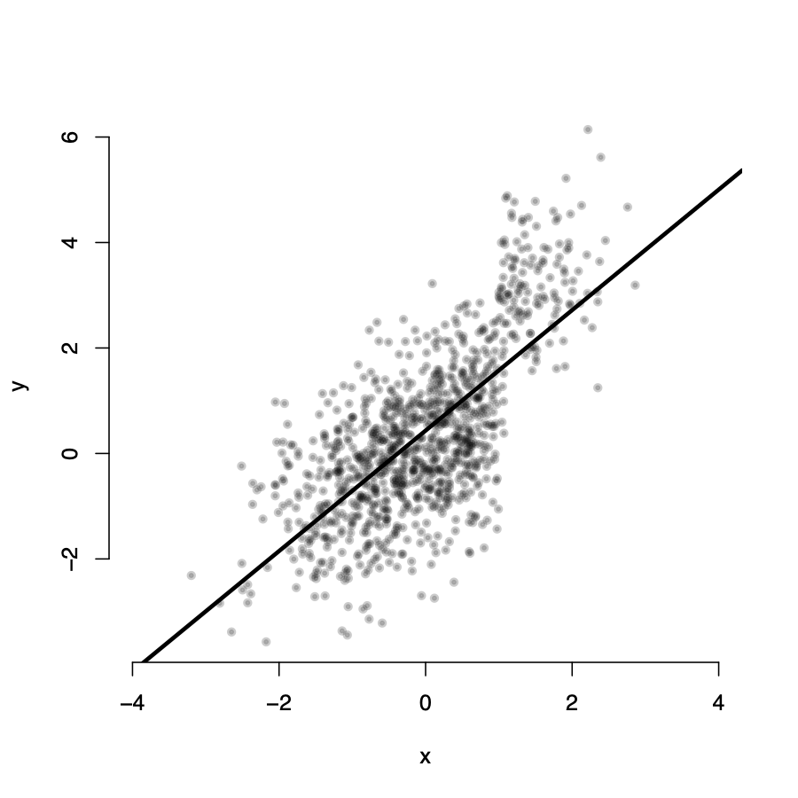
Assumption 1: \(E(u_i|X_i) \neq 0\)
Assumption 1: \(E(u_i|X_i) \neq 0\)

\(Y_i\) is not randomly distributed around the line for all values of X
\(\rightarrow\) the expected value of \(u_i\) is not zero for all \(X_i\) values
\(\rightarrow\) it seems we have omitted an important variable from our model
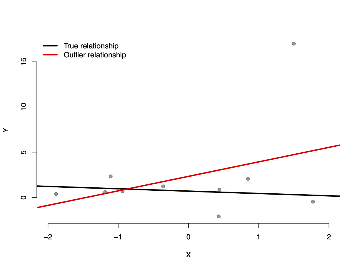
Assumption 3: Large outliers are unlikely
Misspecification of the functional form
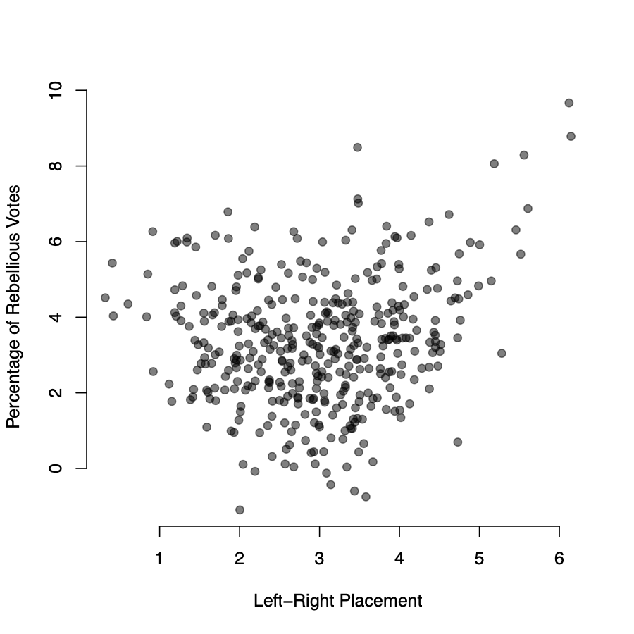
Misspecification of the functional form
- We under-predict the rebelliousness of extremists
- We over-predict the rebelliousness of centrists
- The partial relationship between left-right placement and rebellion is clearly nonlinear
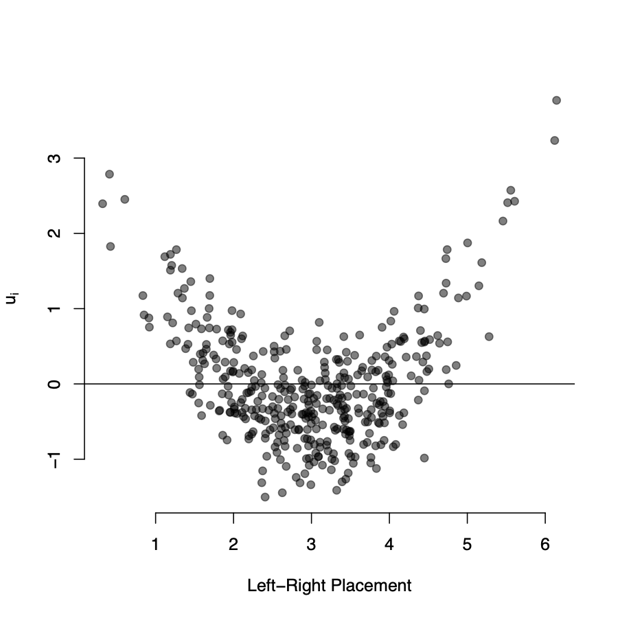
Misspecification of the functional form
Let’s plot the residuals from model 2 against the L-R variable:
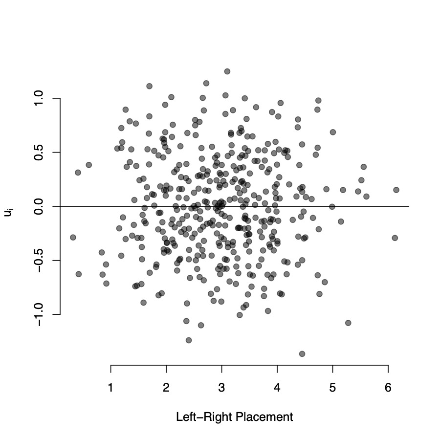
- The residuals are randomly distributed around zero
- There is no detectable “pattern” in the residuals
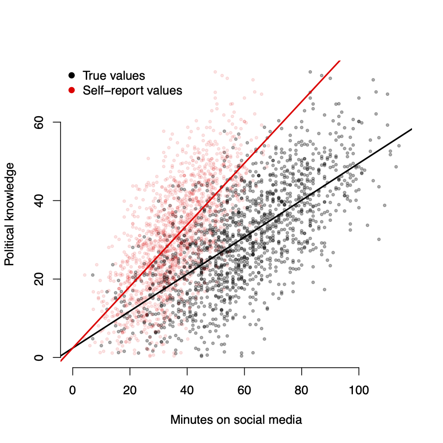
Measurement errors
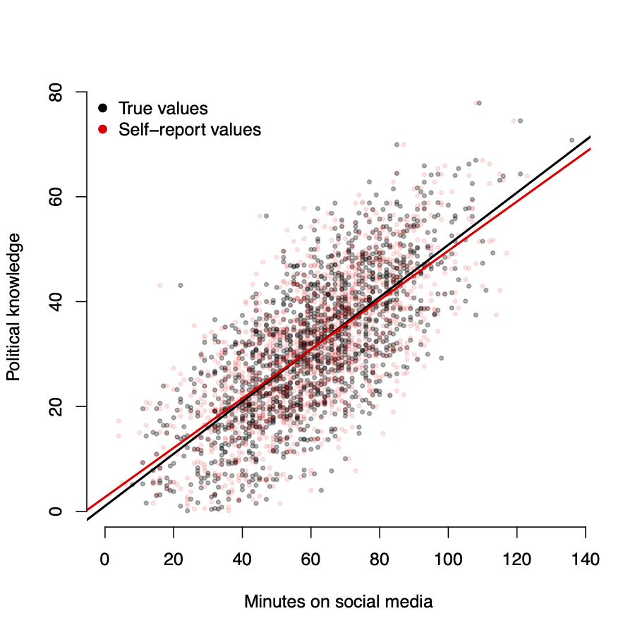
- Black \(\rightarrow\) true values of \(X\)
- Red \(\rightarrow\) reported values of \(\tilde{X}\)
- \(w_i \sim N(0, 5)\)
As measurement error increases, \(\hat{\beta}\) \(\rightarrow\) 0
Measurement errors
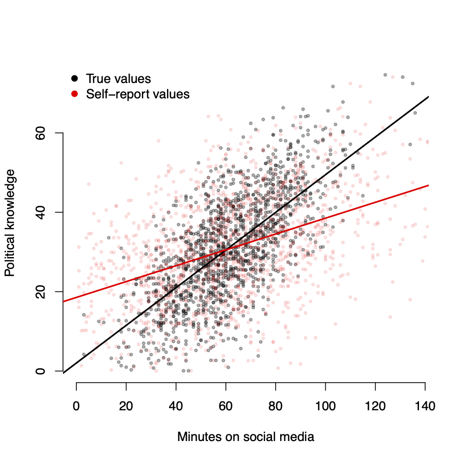
- Black \(\rightarrow\) true values of \(X\)
- Red \(\rightarrow\) reported values of \(\tilde{X}\)
- \(w_i \sim N(0, 15)\)
As measurement error increases, \(\hat{\beta}\) \(\rightarrow\) 0
Measurement errors
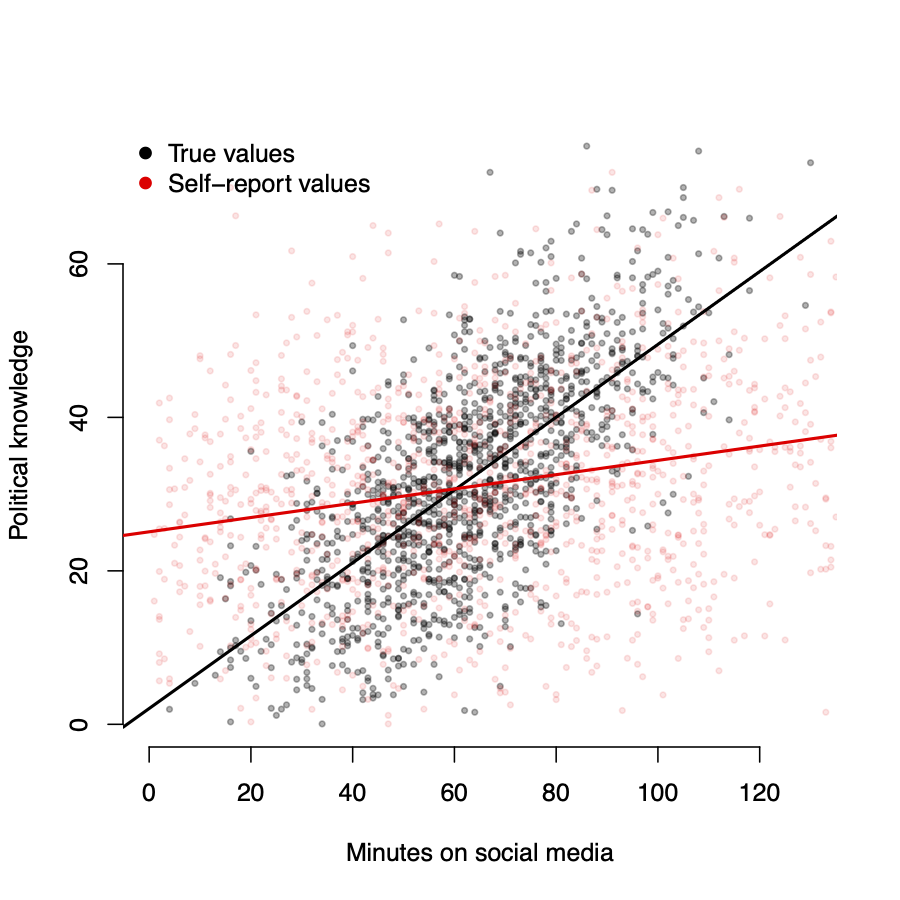
- Black \(\rightarrow\) true values of \(X\)
- Red \(\rightarrow\) reported values of \(\tilde{X}\)
- \(w_i \sim N(0, 25)\)
As measurement error increases, \(\hat{\beta}\) \(\rightarrow\) 0
Measurement errors
More likely is that respondents make systematic errors in stating the amount of time they spend on social media
- Imagine that all respondents report only 60% of the time they spend on social media:
\[ \tilde{X_i} = X_i*.60 \]
- \(\hat{\beta}\) will be biased up by 40%
If the error is non-random, \(\hat{\beta}\) will also be biased
Missing data and sample selection
Let’s assume that people with low levels of political knowledge are on average less likely to respond to political surveys.
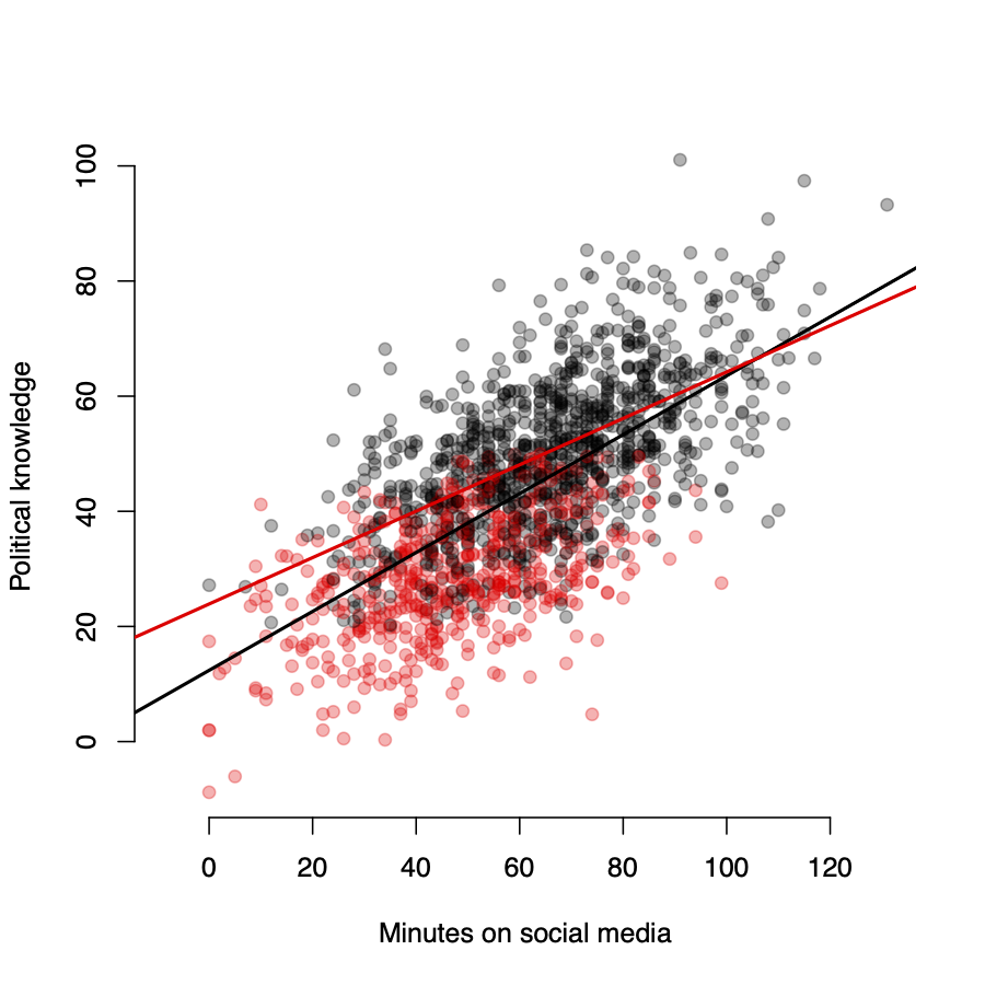
- Black \(\rightarrow\) observations in sample
- Red \(\rightarrow\) observations excluded from sample
- \(\hat{\beta}\) is biased downwards
If sample selection is based on Y, \(\hat{\beta}\) will also be biased
Homoskedasticity vs Heteroskedasticity
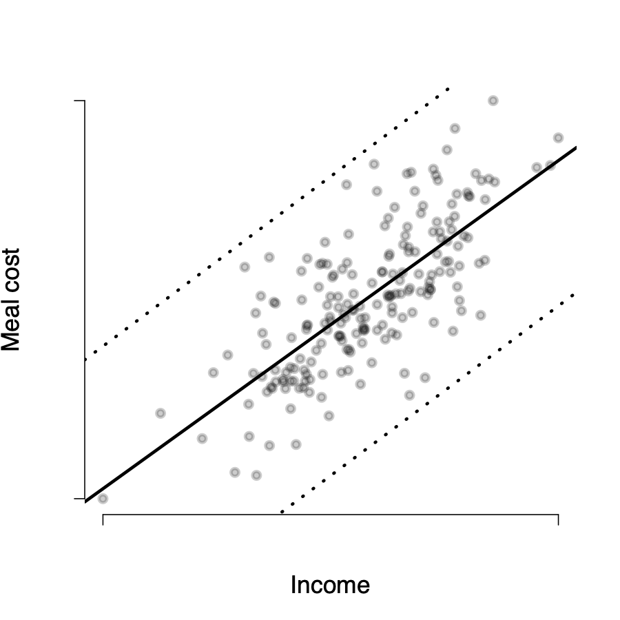
\(Var(u_i | X_i=x)=\)const.
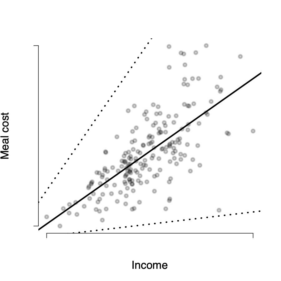
\(Var(u_i | X_i=x)\neq\)const.
Detecting heteroskedasticity visually
We can detect heteroskedasticity visually by again plotting the residuals against our X variables:
\(\rightarrow\) when the distribution of \(u_i\) follows this “funnel” shape, that suggests the errors are heteroskedastic