POL272 Quantitative Methods for Social Science Research
Sebastian Koehler
2026-02-19
Notes on the midterm assessment
Assessment is a research project, that will take the shape of a 3-minute TikTok-style video. You will need to submit the video alongside a script and the R code. The maximum limit is 2,000 words - this is a limit, not a goal.
Instructions and data were posted today and we will dedicate a section of the Lecture to discuss them
You will have to submit on QMPlus, assignment is due on 10 March 2026
The assessment will comprise a series of tasks, which will require you to manipulate data and produce output using RStudio
Pro-tip: the practical tasks are the same ones you have done in the seminars.
Why do we analyse data?
MEASURE:To infer population characteristics via survey research
what proportion of constituents support a particular policy?
PREDICT:To make predictions
who is the most likely candidate to win an upcoming election?
EXPLAIN:To estimate the causal effect of a treatment on an outcome
what is the effect of small classrooms on student performance?
Plan for today
Sample vs. Population
Representative samples
Random Sampling
Random Treatment Assignment vs. Random Sampling
Exploring One Variable At a Time
Table of frequencies
Table of proportions
Histogram
Descriptive Statistics: mean, median, standard deviation, and variance
Exploring the Relationship Between Two Variables
Scatter plots
Correlations
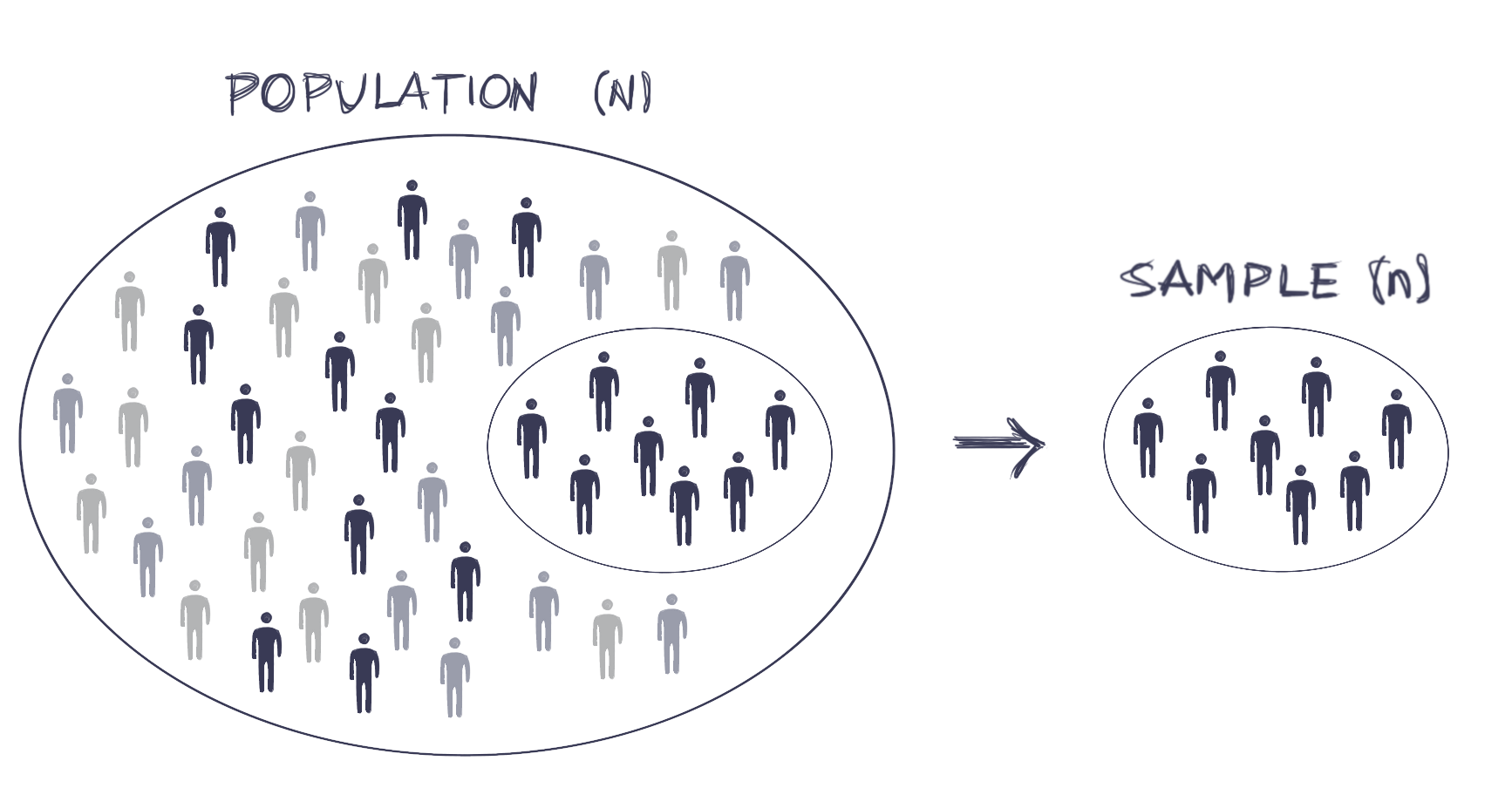
Sample vs. Population
We often want to know the characteristics of a large population such as the residents of a country
Yet collecting data from every individual in the population is either prohibitively expensive or simply infeasible
In the UK, we try to collect data from each individual every ten years
The 2021 census cost £1 billion, approximately (population at that time was around 60 million)
This is not feasible for research purposes!
We use surveys to collect data from a small subset of observations in order to understand the population
Subset of individuals chosen for study is called a sample
In the UK, researchers typically survey only about 1,200 people to infer the characteristics of more than 35 million adult citizens (n=1,200, N=35 million)
Representative Samples
In survey research, it is vital for the sample to be representative of the population of interest
A representative sample accurately reflects the characteristics of the population from which it is drawn, that is, characteristics appear in the sample in similar proportions as in the population as a whole
If the sample is not representative, our inferences regarding the population characteristics based on the sample will be wrong
Are you a representative sample of UK residents?
Are you a representative sample of QMUL students?
Are you a representative sample of QMUL Politics and IR students?
Are you a representative sample of POL272 students?
What would be the best way to draw a representative sample of QMUL students?
using random sampling
get the list of all QMUL students and select n students at random
Random Sampling
The best way to draw a representative sample is to select individuals at random from the population
This procedure is called random sampling
Random sampling
makes the sample and the target population on average identical to each other in all observed and unobserved characteristics
Random sampling ensures that the sample is representative of the target population
enabling us to infer valid population characteristics from the sample
Random Treatment Assignment vs. Random Sampling
Do not confuse them with each other: they both use a random process but for two very different reasons
Random treatment assignment means that the treatment is assigned at random
makes treatment and control groups comparable
enables us to produce valid estimates of the average treatment effect (using diffs-in-means estimator)
Random sampling means that individuals are selected at random from the population into the sample
makes sample representative of the population
enables us to infer valid population characteristics from the sample
Exploring One Variable At a Time
Suppose we have collected data from a sample, now what?
To understand the content and distribution of each variable we can
create a table of frequencies
create a table of proportions
create a histogram
compute descriptive statistics
Let’s return to the voting experiment
data collected from a sample of registered voters in the state of Michigan
The voting dataset
Unit of observation: Registered voters
Variables:
Variable
Description
birth
year of birth
message
whether registered voter received the message (“yes” or “no”)
voted
whether registered voter voted: 1= yes; 0=no
In-Class Exercise
Open RStudio
Download exercise_3.R from the module’s website and open it within RStudio
Run steps 1 through 3
Explore one variable at a time
follow along
## STEP 1. Set the working directorysetwd("~/Desktop/POL272") # example if Mac setwd("C:/user/Desktop/POL272") # example if Windows
## STEP 2. Load the datasetvoting <-read.csv("voting.csv") # reads and stores data
## STEP 3. Look at the datahead(voting) # shows the first six observations## birth message voted## 1 1981 no 0## 2 1959 no 1## 3 1956 no 1## 4 1939 yes 1## 5 1968 no 0## 6 1967 no 0## what's the unit of observation?## for each variable: type and unit of measurement?## substantively interpret the first observation
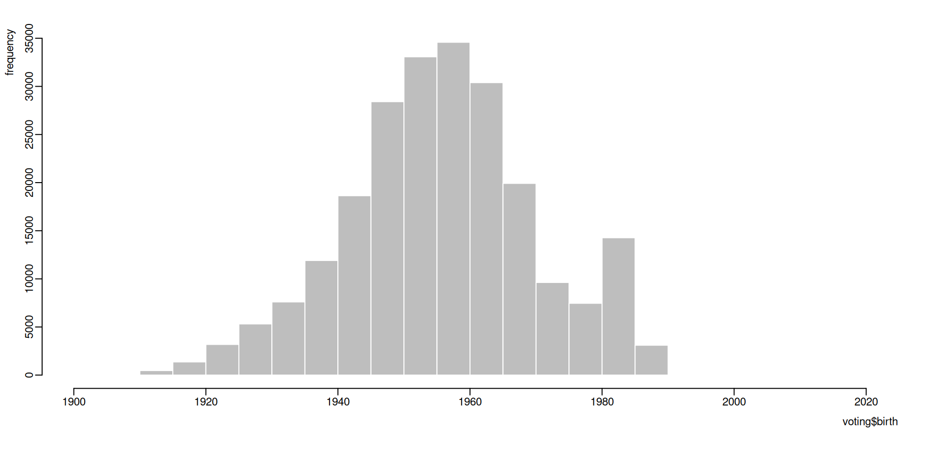
Table of Frequencies
The frequency table of a variable shows the values the variable takes and the number of times each value appears in the variable
\(sd(X)\) stands for the standard deviation of \(X\)
\(X_i\) is a particular observation of \(X\)
\(\overline{X}\) stands for the mean of \(X\)
\(n\) is the total number of observations in the variable
\(\sum^{n}_{i=1} (X_i{-}\overline{X})^2\) means the sum of all \((X_i{-}\overline{X})^2\) from \(i{=}1\) to \(i{=}n\)\
Important
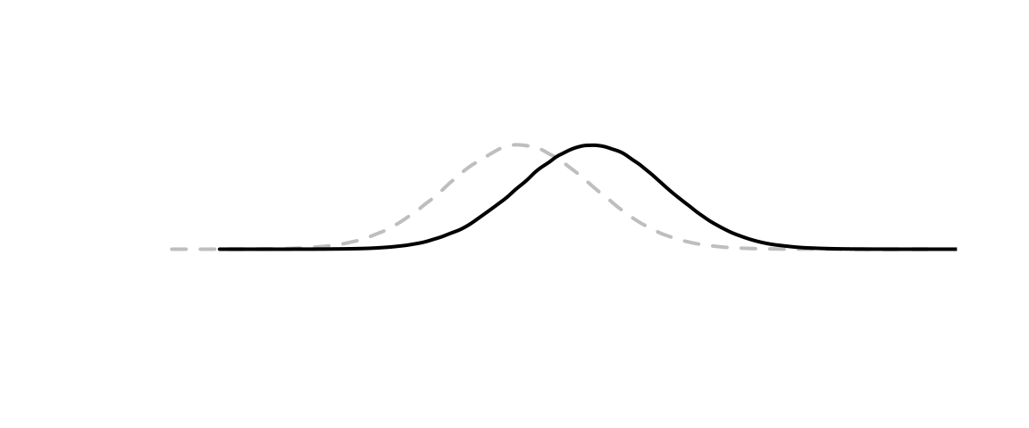
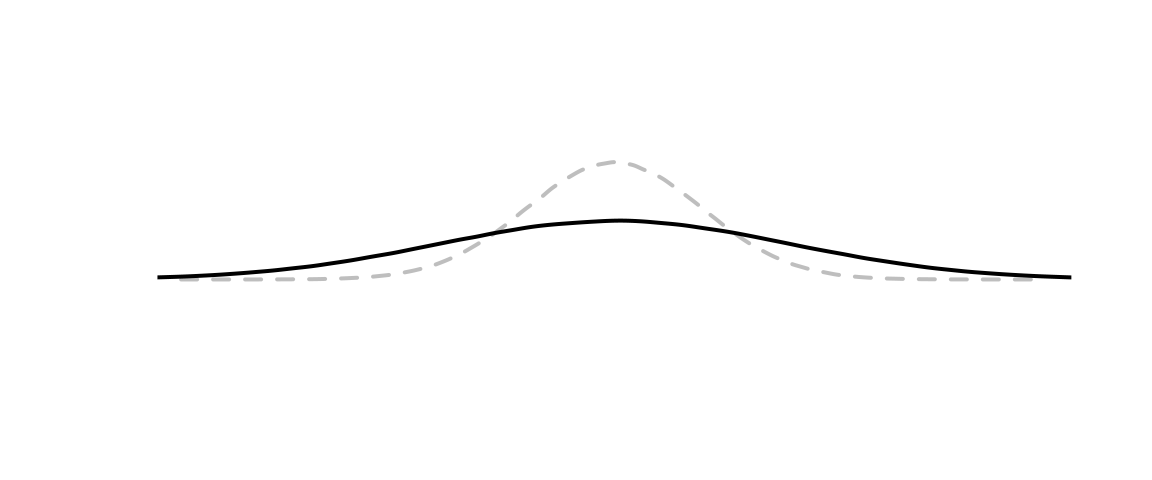
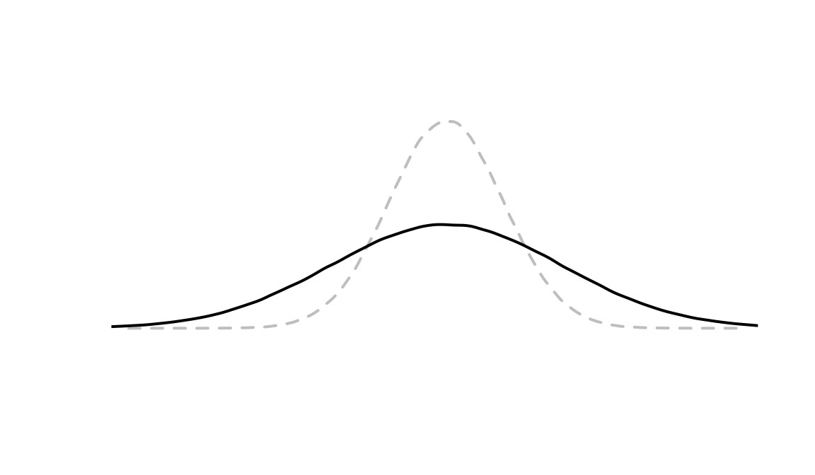
The standard deviation of a variable measures the average distance of the observations to the mean.
The larger the standard deviation,
the flatter the distribution
Which distribution has a larger standard deviation?
The standard deviation of a variable gives us a sense of the range of the data, especially when dealing with bell-shaped distributions known as normal distributions
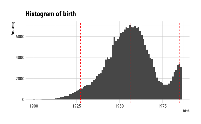
In normal distributions, 95% of the observations fall within two standard deviations from the mean
R function: sd()
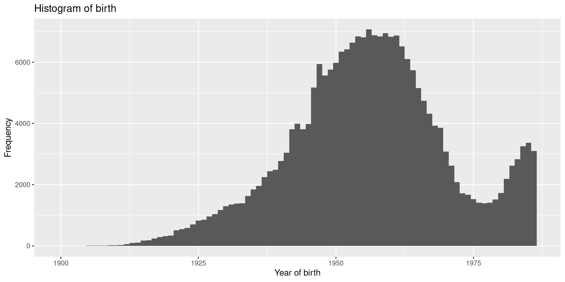
sd(voting$birth)
[1] 14.46019
If birth were normally distributed, about 95% of the registered voters in the voting experiment would have been born between 1927 and 1985
The variance of a variable is simply the square of the standard deviation \[var(X) = sd(X)^2\]
\(var(X)\) stands for the variance of \(X\)
\(sd(X)\) stands for the standard deviation of \(X\)
R function: var()
var(voting$birth)
[1] 209.0971
Alternatively: sd()\^{}2
sd(voting$birth)^2
[1] 209.0971
We are usually better off using standard deviations as our measure of spread, as they are easier to interpret because they are in the same unit of measurement as the variable
If we are given a variance, we can compute the standard deviation by taking the square root of the variance.
What is the R function to compute a square root?
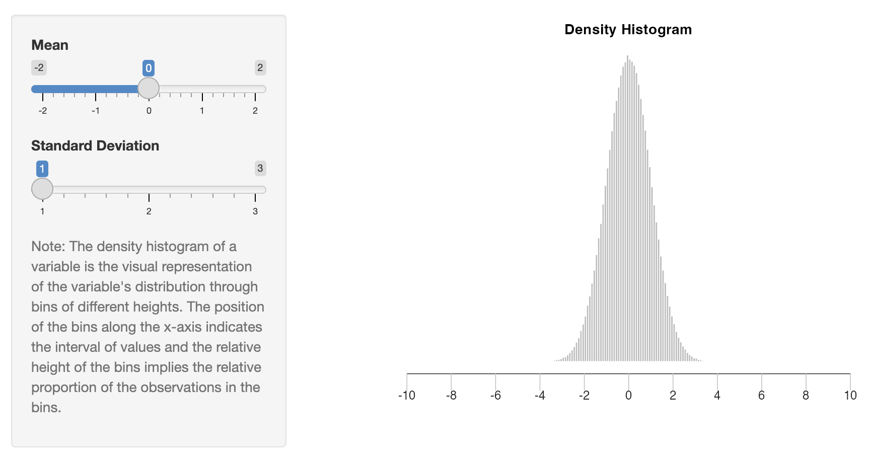
Understanding How the Mean and the Standard Deviation of a Variable Change the Variable’s Distribution (link to interactive graph)
Understanding the relationship between two variables
We saw how to explore one variable at a time
creating table of frequencies and/or proportions
creating histograms
computing descriptive statistics: mean, median, standard deviation, and variance
Most data analyses are about understanding the relationship between two variables
To explore the relationship between two variables we
create scatter plots
compute correlation coefficient
Scatter Plots
A scatter plot enables us to visualize the relationship between two variables by plotting one variable against the other in the two-dimensional space
Imagine we have two variables:
X
Y
4
2
8
5
10
3
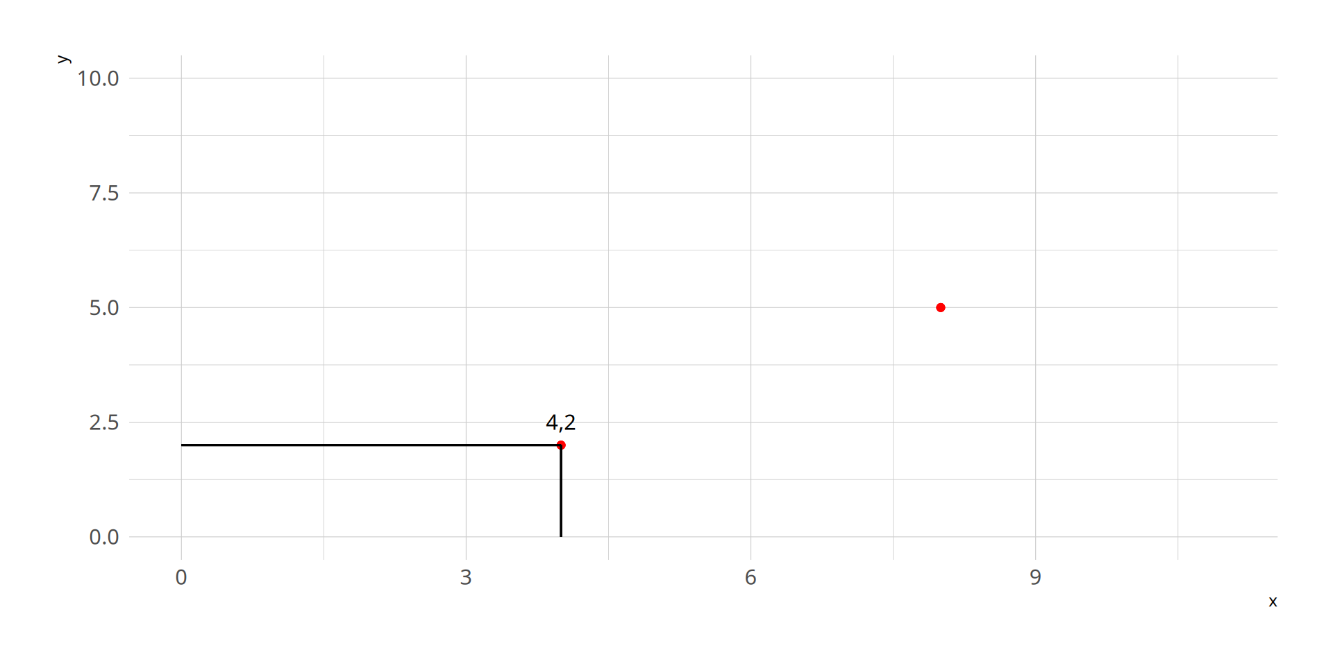
We can create the scatter plot by plotting one layer at a time:
Imagine we have two variables:
X
Y
4
2
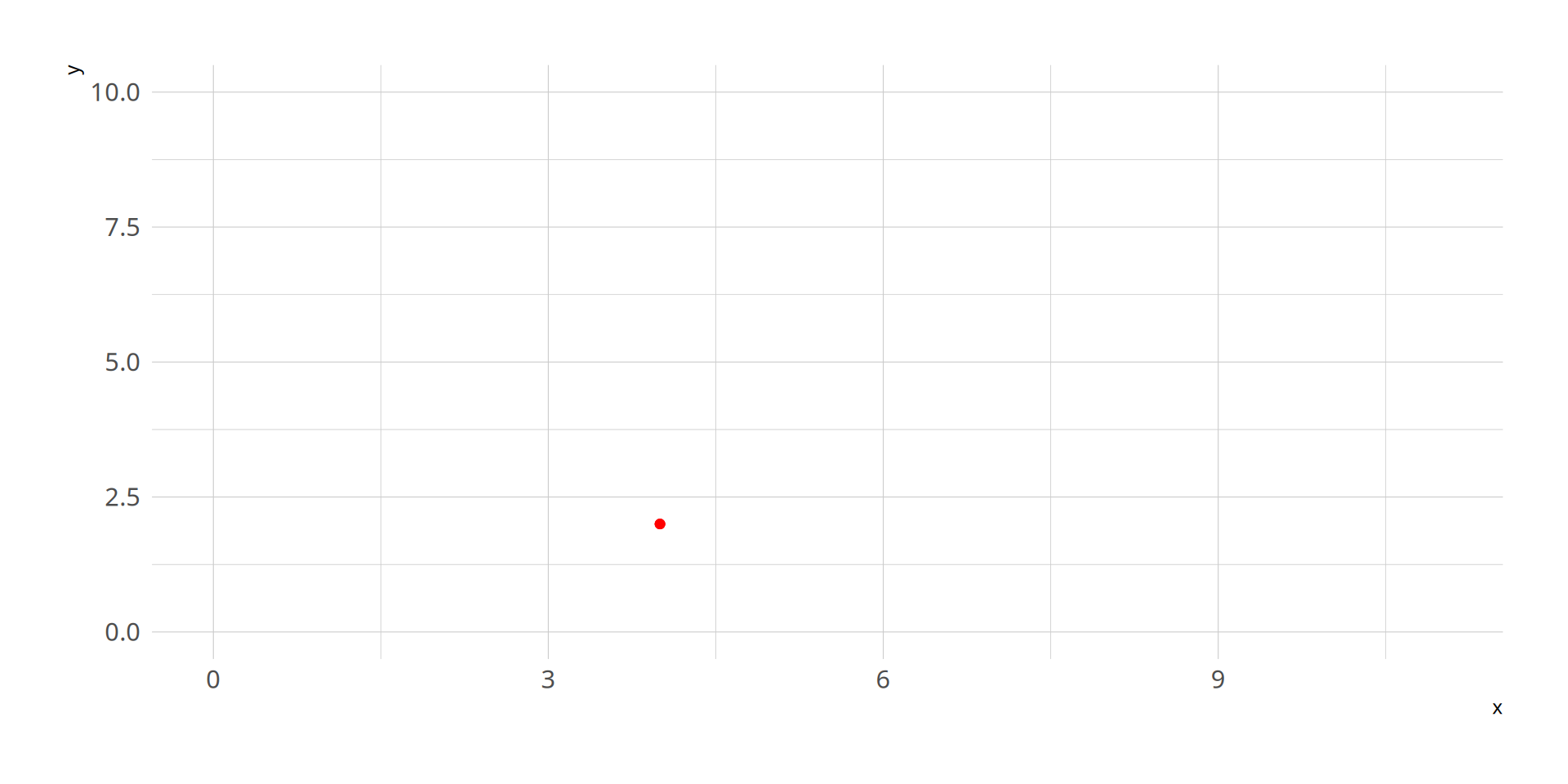
First, let’s plot this point:(\(x_1\), \(y_1\)) = (4,2)
8
5
10
3
We can create the scatter plot by plotting one layer at a time:
Imagine we have two variables:
X
Y
4
2
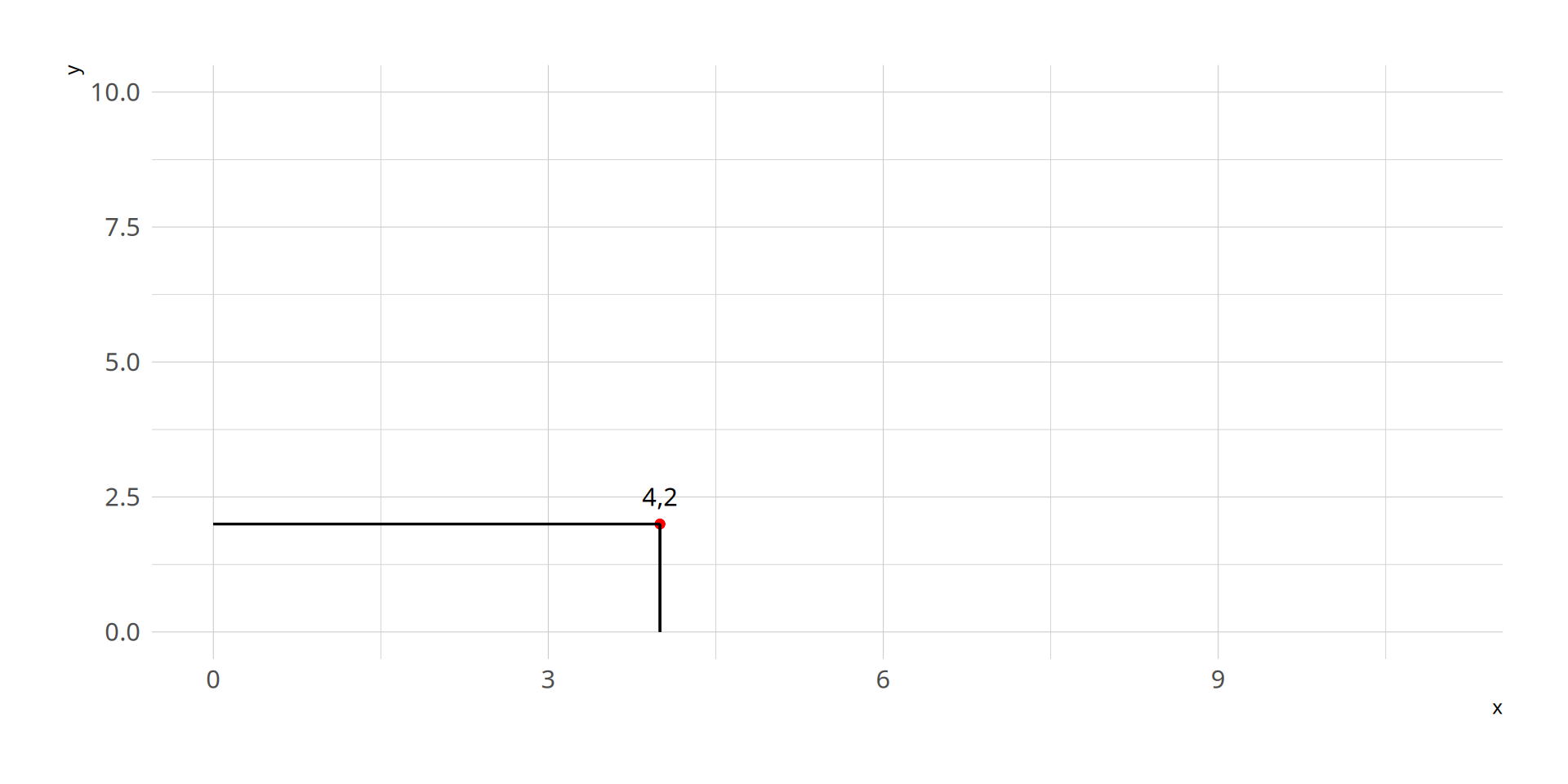
First, let’s plot this point:(\(x_1\), \(y_1\)) = (4,2)
8
5
10
3
We can create the scatter plot by plotting one layer at a time:
Imagine we have two variables:
X
Y
4
2
First, let’s plot this point:(\(x_1\), \(y_1\)) = (4,2)
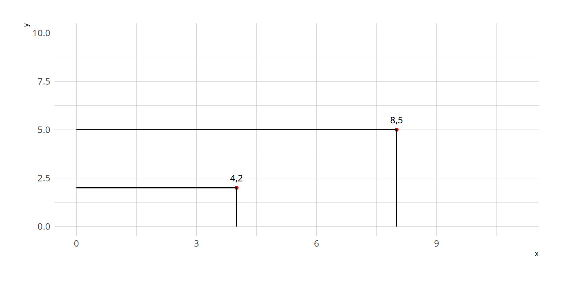
8
5
Now, let’s plot this point:(\(x_2\), \(y_2\)) = (8,5)
10
3
We can create the scatter plot by plotting one layer at a time:
Imagine we have two variables:
X
Y
4
2
First, let’s plot this point:(\(x_1\), \(y_1\)) = (4,2)
8
5
Now, let’s plot this point:(\(x_2\), \(y_2\)) = (8,5)
10
3
We can create the scatter plot by plotting one layer at a time:
Imagine we have two variables:
X
Y
4
2
First, let’s plot this point:(\(x_1\), \(y_1\)) = (4,2)
8
5
Now, let’s plot this point:(\(x_2\), \(y_2\)) = (8,5)
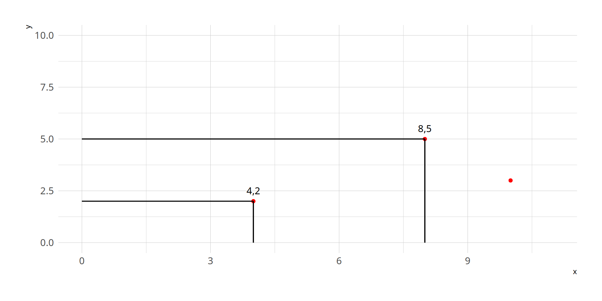
10
3
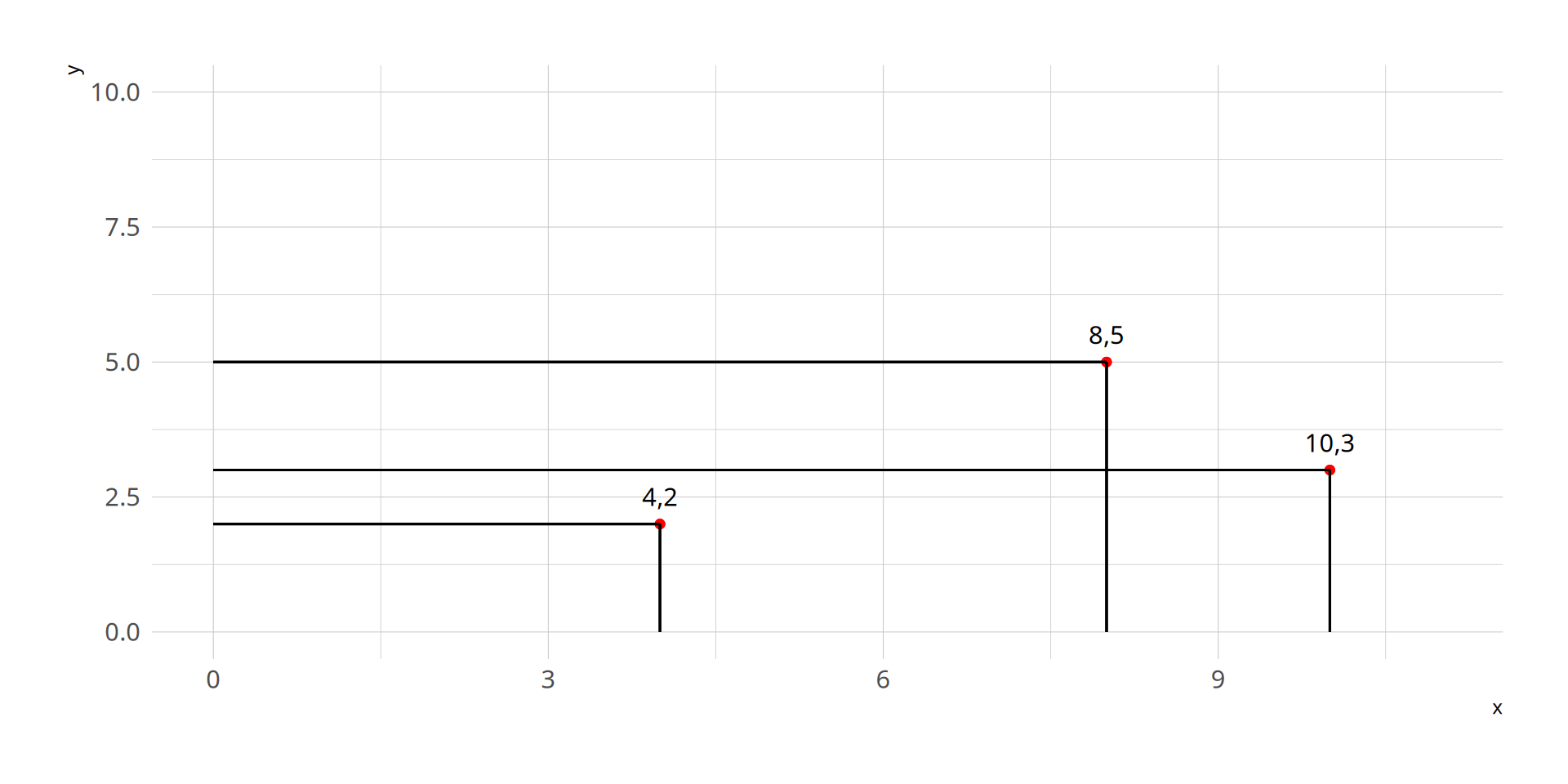
Finally, let’s plot:(\(x_3\), \(y_3\)) = (10,3)
We can create the scatter plot by plotting one layer at a time:
Imagine we have two variables:
X
Y
4
2
First, let’s plot this point:(\(x_1\), \(y_1\)) = (4,2)
8
5
Now, let’s plot this point:(\(x_2\), \(y_2\)) = (8,5)
10
3
Finally, let’s plot:(\(x_3\), \(y_3\)) = (10,3)
We can create the scatter plot by plotting one layer at a time:
R function: ggplot()
How many arguments are required?
two; the two variables
Enter arguments in the expected order: first X, second Y
ggplot( aes(x,y))
Then the rest of the layers:
geom_point(), annotate(), segment()
Let’s use the data from Project STAR:
star <-read.csv("STAR.csv") # reads and stores datahead(star) # shows first observations
  classtype reading math graduated
1     small     578  610         1
2   regular     612  612         1
3   regular     583  606         1
4     small     661  648         1
5     small     614  636         1
6   regular     610  603         0
Unit of observation?
students; each observation represents a student
Unit of measurement of reading and math?
points
What would be the code to create the scatter plot between reading and math, where reading is on the x-axis and math is on the y-axis?
Answer:
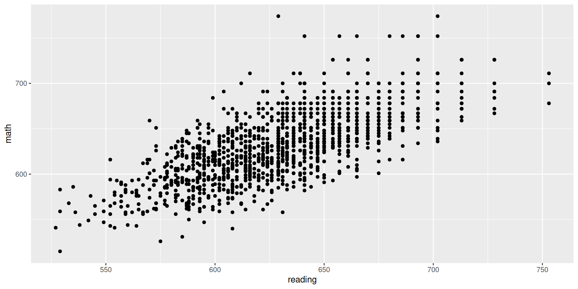
star |>ggplot(aes(x = reading, y = math)) +geom_point()
What can we learn from this scatter plot about the relationship between these two variables?
Are students who tend to do well in one exam also tend to do well in the other?
Correlation Coefficient
The correlation coefficient or correlation is a statistic that summarizes the relationship between two variables, X and Y, with a number
denoted as cor(X,Y) in mathematical notation
It summarizes the direction and strength of the linear association between the two variables
cor(X,Y) ranges from -1 to 1
The sign reflects the direction of the linear association:
cor(X,Y) > 0 if the slope of the line of best fit is positive
cor(X,Y) < 0 if the slope of the line of best fit is negative
The absolute value reflects the strength of the linear association:
|cor(X,Y)| = 0 if there is no linear association
|cor(X,Y)| = 1 if there is a perfect linear association
|cor(X,Y)| increases as the observations move closer to the line of best fit and the linear association becomes stronger
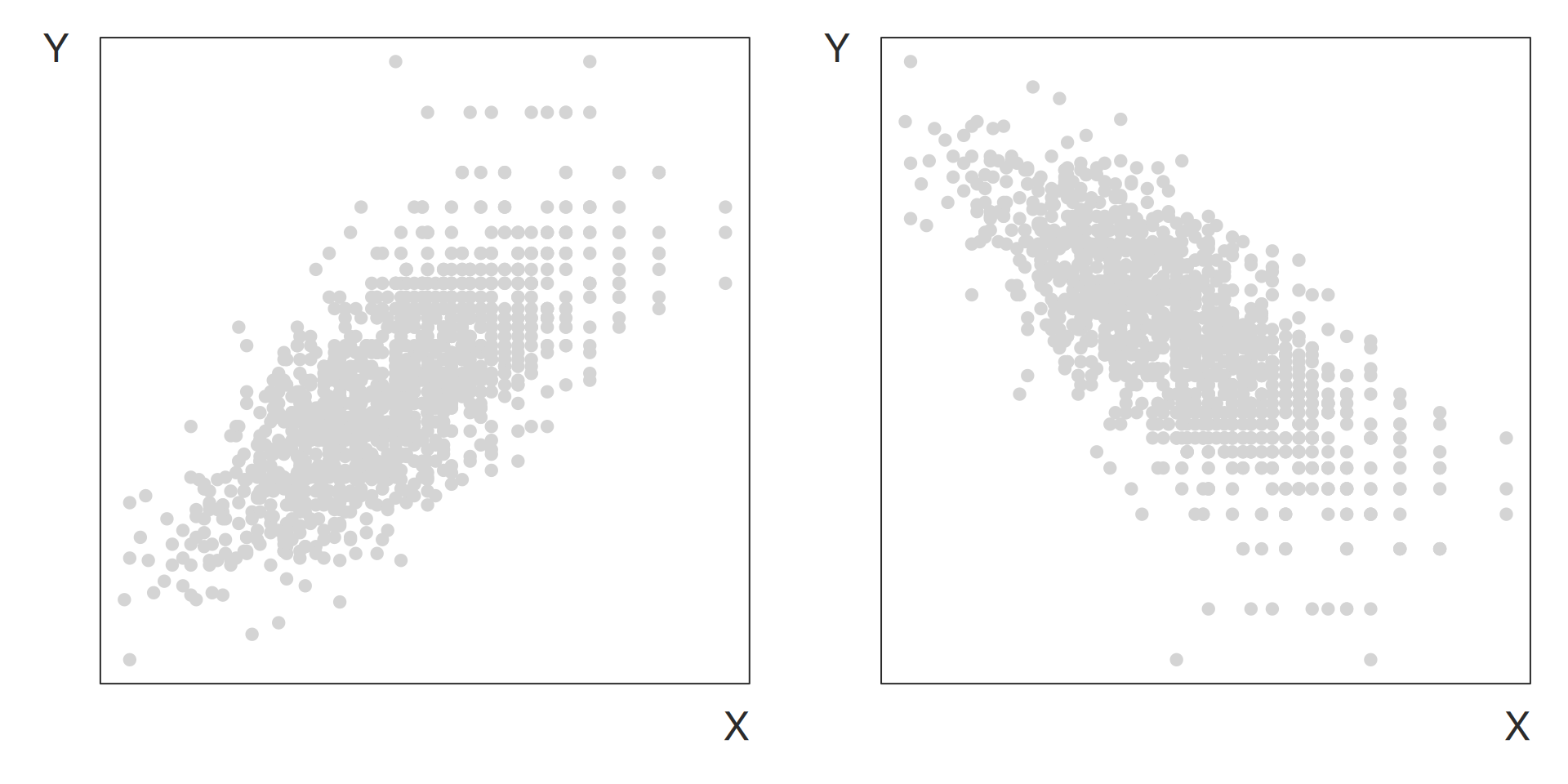
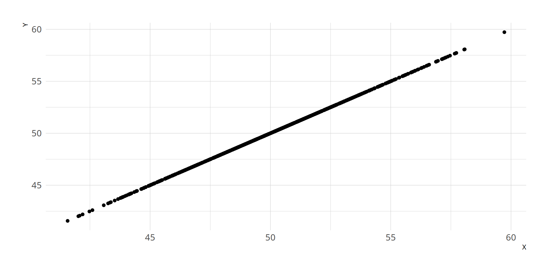
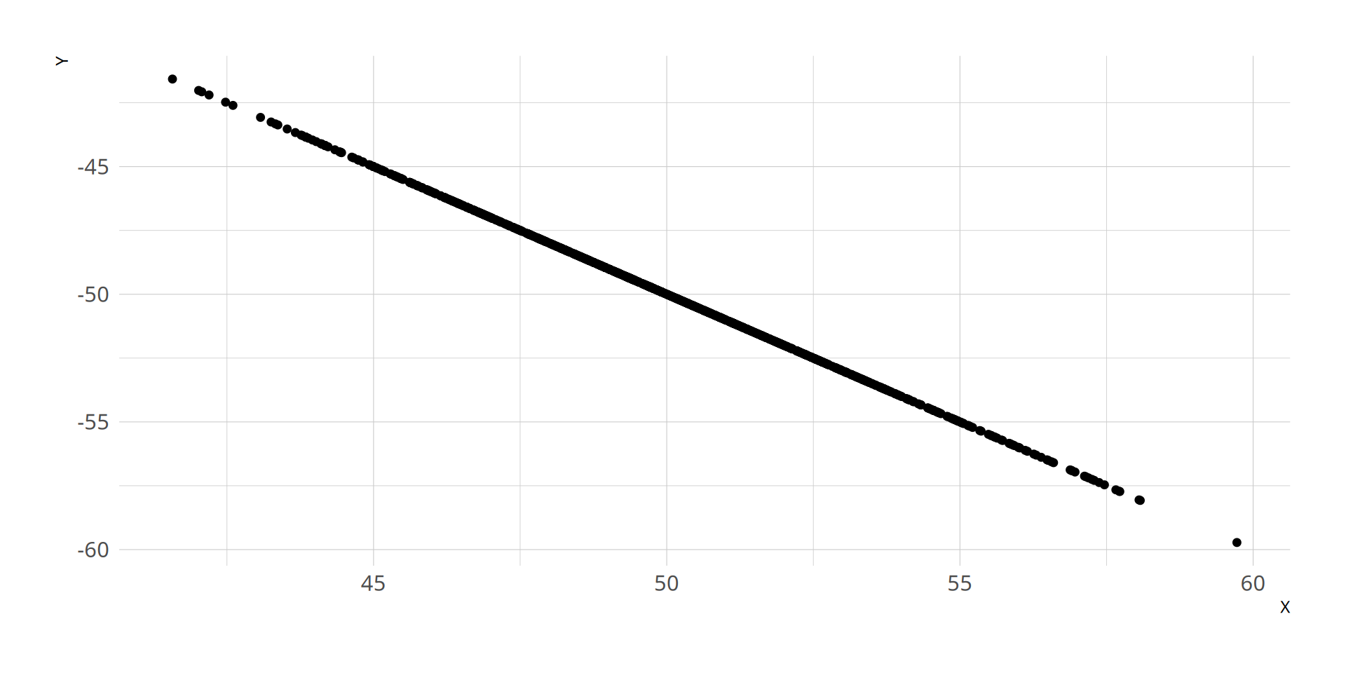
Example of change in direction of the linear association between two variables:
positive linear association
negative linear association\positive
correlation
negative correlation
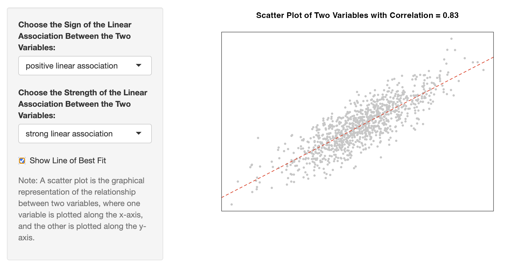
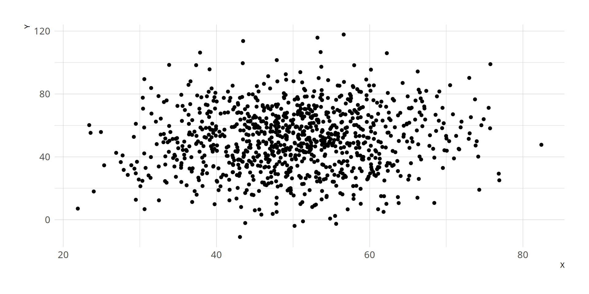
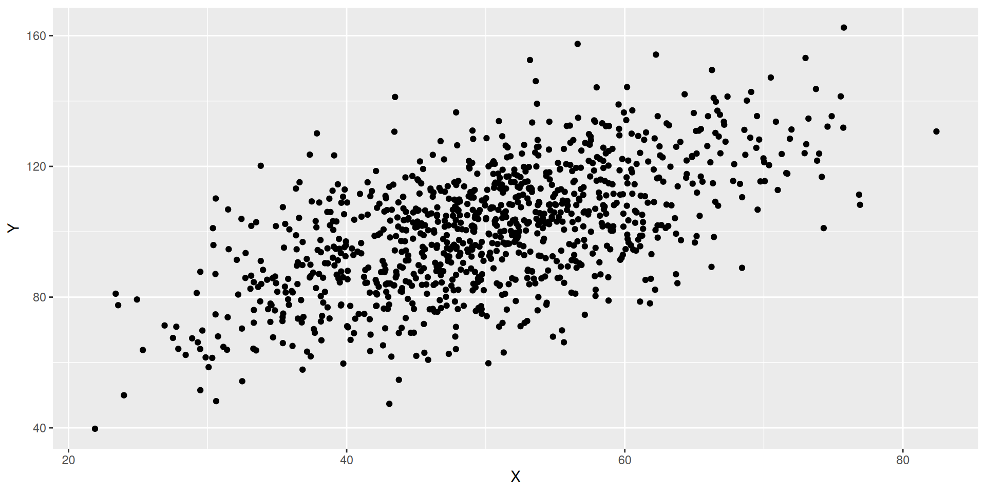
Example of change in strength of the linear association between two variables:
weak linear association
strong linear association\positive
absolute value close to 0
absolute close to 1
Understanding the Two Characteristics the Correlation Coefficient Captures (link to interactive graph)
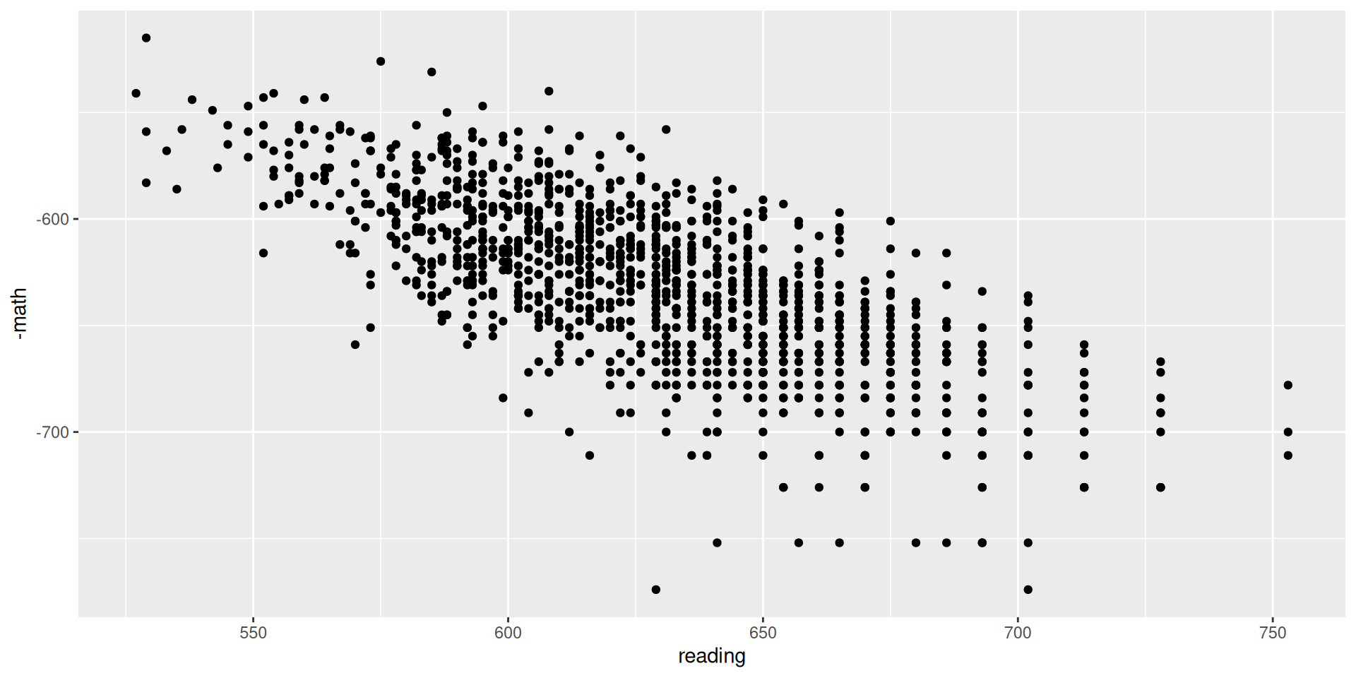
Is the slope of the line of best fit positive or negative?
Do you expect the correlation between reading and math to be positive or negative?
Does the association look strongly linear?
Do you expect the absolute value of the correlation between reading and math to be closer to 1 or to 0?
R function: cor()
How many required arguments?
two; the two variables
Does the order of the arguments matter?
no; cor(X,Y) = cor(Y,X)
What’s the code to compute the correlation between reading and math?
Answer:
cor(star$math, star$reading)
[1] 0.7161218
# ORcor(star$reading, star$math)
[1] 0.7161218
Is the correlation what we expected?
sign of slope of best line? ___
strong linear association? ___
cor(X,Y) = ___
sign of slope of best line? ___
strong linear association? ___
cor(X,Y) = ___
sign of slope of best line? ___
strong linear association? ___
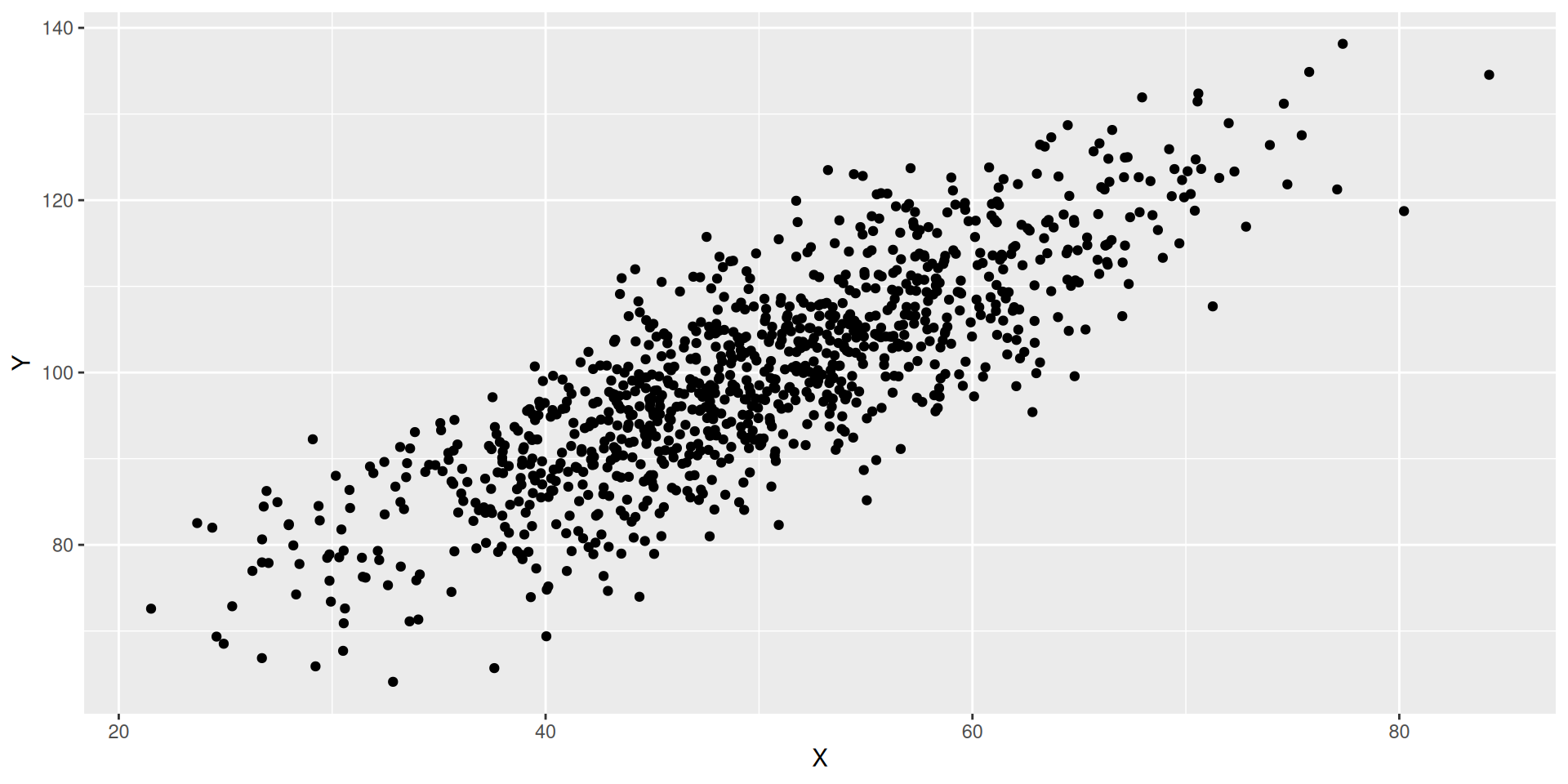
cor(X,Y)\(\approx\) ___
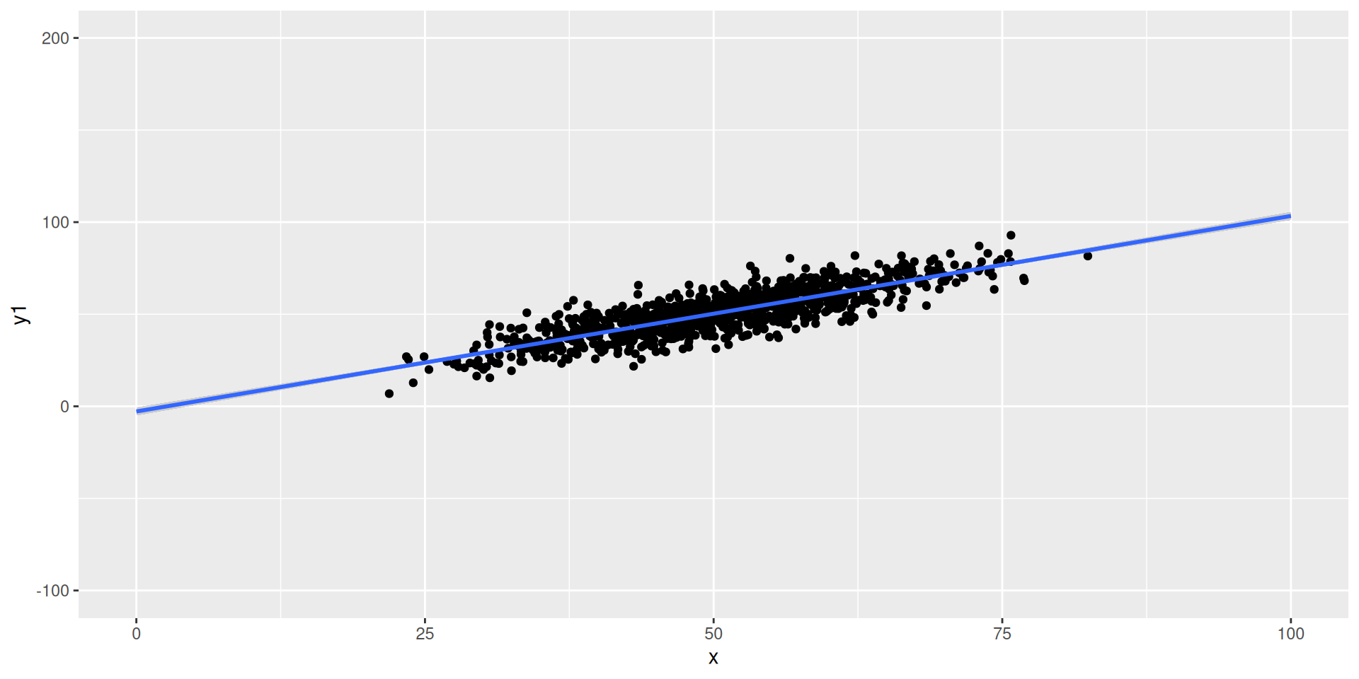
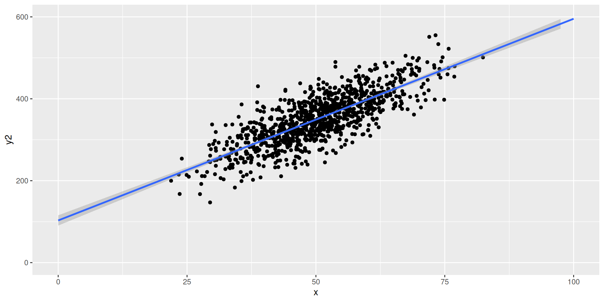
The correlation in the second scatter plot is _______ (higher/lower) than the correlation in the first scatter plot
line of best fit is steeper in ___ (first/second) scatter plot- correlation is higher in ___ (first/second) scatter plot
A steeper line of best fit does not necessarily mean a higher correlation in absolute terms, or vice versa
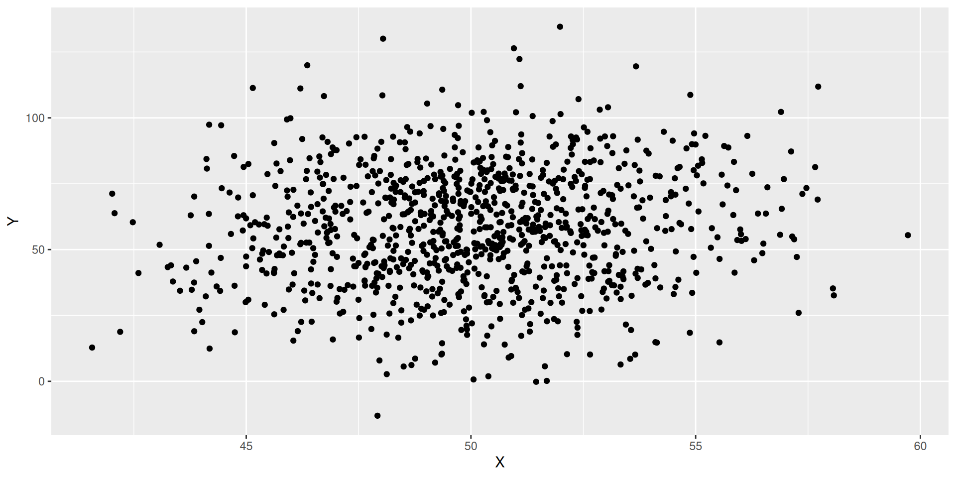
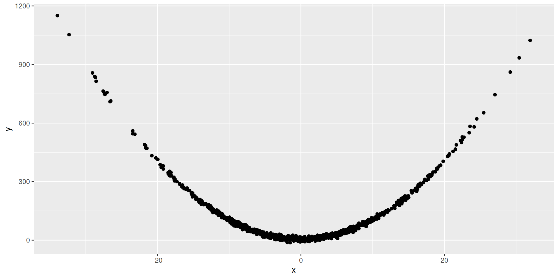
cor(X,Y) \(\approx\) 0. Does this mean that there is no relationship between the two variables?
No, it just means that there is no linear relationship between the two variables
If two variables have a correlation of zero, it does not necessarily mean that there is no relationship between them
Correlation does not necessarily imply causation
Just because two variables have a strong linear association does not mean that changes in one variable cause changes in the other
reading and math are highly correlated with each other: doesn’t mean that an improvement on your reading scores will cause an improvement on your math scores